| Table of Contents |
Crummett and Western, Physics: Models and Applications,
Sections 14-2, 5
Halliday, Resnick, and Walker, Fundamentals of Physics (5th
ed.), Sections 16-2, 3, 8, 9
Tipler, Physics for Scientists and Engineers (3rd ed.), Sections
12-1, 7, 8
This laboratory will let you perform some simple experiments with an oscillating mechanical system consisting of a spring and a mass. You will observe and analyze free vibration, where the system is given an initial displacement, and then left to vibrate "on its own." You will also study forced vibration, where the system is driven by an external sinusoidal input force. A common objective of both approaches is to calculate the value of a critical parameter: the elastic constant of the system spring. The values that you get for "k" in the two cases will be compared, and along way, you will observe the primary features of this important type of behavior as exhibited by a mechanical system.
If the net resultant force on a mass m is a linear function of its position x, the resulting motion is a sinusoidal oscillation:
![]() with
with ![]() (1)
(1)
-- but this is never exactly true. (1) describes a motion which goes on unchanging forever, while in any real situation the motion is damped: it dies out with time. One of the simplest models of frictional damping gives
![]() (2)
(2)
 where
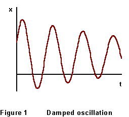
where ![]() The general character of this motion is sketched in Figure 1: the oscillations
damp out as time goes by. (Eventually they will stop.) The "damping
coefficient" d determines the ratio of amplitudes of successive
maxima:
The general character of this motion is sketched in Figure 1: the oscillations
damp out as time goes by. (Eventually they will stop.) The "damping
coefficient" d determines the ratio of amplitudes of successive
maxima:
![]() (3)
(3)
Because of damping in real situations, oscillating systems must be driven
if their motion is to be maintained indefinitely. (A clock pendulum is
driven by the stored potential energy of a raised weight or a wound spring,
a child "pumps" a playground swing, etc.) If an oscillator is
driven by a sinusoidal driving force ![]() ,
the amplitude of the oscillations that result (in a steady state) is
,
the amplitude of the oscillations that result (in a steady state) is
 (4)
(4)
Notice that the amplitude has a maximum at a frequency ![]() near (but not equal to)
near (but not equal to) ![]() and
and ![]() . That is,
you get the biggest response if you drive the oscillator at the frequency
at which it would oscillate freely. This phenomenon is called resonance.
. That is,
you get the biggest response if you drive the oscillator at the frequency
at which it would oscillate freely. This phenomenon is called resonance.
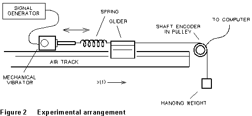
A schematic drawing of your experiment is shown below. As long as the string connecting the glider and the hanging mass remains taut, these two objects move together; together they comprise the oscillating system. The string and hanging mass are included so that the linear motion of the system is

translated 1:1 into rotational motion of the pulley; rotation of the
pulley rotates the shaft encoder attached to its axle, and the angular
displacement ![]() of
the pulley is recorded by the computer. This angular displacement is related
to the linear motion of the system by x(t) = R
of
the pulley is recorded by the computer. This angular displacement is related
to the linear motion of the system by x(t) = R![]() (t),
where R is the pulley radius. The purpose of most of the equipment
in the sketch is to allow this automated data recording. The mechanical
vibrator is used to drive the system. Where do you think the damping
in this system comes from?
(t),
where R is the pulley radius. The purpose of most of the equipment
in the sketch is to allow this automated data recording. The mechanical
vibrator is used to drive the system. Where do you think the damping
in this system comes from?
(1) Remove the signal generator connection from the mechanical vibrator. Lock the mechanical vibrator via the Lock/Unlock switch on the mechanism. Set up the spring, glider, and hanging weights as shown in Figure 2. Turn on the air to the track, and slowly increase the hanging weight until the spring is stretched 2 to 4 cm. This weighting/stretching is critical! Check to see that the oscillations are smooth.
(2) GENTLY, remove and weigh the cart mass and the hanging masses. These two masses together are the "oscillating mass."
(3) You will use the shaft encoder and your computer to record and measure the displacement of the system. The responses will then be analyzed to discover the spring coefficient. You will need to remember some of what you have learned about the shaft encoders from the previous labs. Make several measurements of the radius of the encoder.
(4) Be sure the mechanical vibrator is off. Set the software to take 2000 points, recording every 5th point. Enter the radius of your shaft encoder wheel into the program.
(5) Displace the slider mass so as to stretch the spring by about 2 cm. Release the system from rest as carefully as possible, simultaneously keying the data taking option on the computer. Have the system go through enough cycles of oscillation so that its amplitude is about 25-30% of the original value. Plotting should give something like Figure 1. Save your data to a file for further analysis.
(6) Briefly examine the "phase plot" of the system by plotting x against its derivative, v. Roughly sketch what you see in your laboratory notebook, labeling and commenting upon any important features.
(7) Display the position vs. Time data. Record the maximum amplitude
A from the left side of the display. Expand the display from the first
minimum or maximum to the last minimum or maximum respectively so that
you are displaying an integral number of cycles. Calculate the elapsed
time for these cycles from the horizontal axis of the display. Calculate
the period (T = elapsed time/number of cycles), of the oscillations and
the damped angular frequency ![]() .
.
Use equation (3) to calculate/estimate the damping coefficient, d, using the ratio of amplitudes at successive peaks.
You can now use the software to fit equation (2) to your data. Make
sure your data has been re-expanded to view the full data set. Select the
sine wave fit. You should have good estimates of all of the parameters
in equation (2) from the calculations you have just done with the exception
of the phase constant,![]() ,
which is unique for each starting time. Input your parameter into the equation
on the computer.
,
which is unique for each starting time. Input your parameter into the equation
on the computer.
(8) Adjust ![]() and the other parameters as necessary to get a good fit. This means that
you will have accurate values of d and
and the other parameters as necessary to get a good fit. This means that
you will have accurate values of d and ![]() .
Recalling that
.
Recalling that ![]() and
and ![]() , calculate
the spring constant k. Show all of these calculations and results
in your laboratory notebook.
, calculate
the spring constant k. Show all of these calculations and results
in your laboratory notebook.
(9) (OPTIONAL: CONSULT YOUR INSTRUCTOR.) Repeat the process (5)-(8) for a substantially different value of the hanging mass m. Of course you should get the same value for k (it's the same spring...). Do you, within experimental error?
(10) Now you will drive the system with the mechanical vibrator. Unlock the mechanical vibrator and connect it to the signal generator. Replace the original mass m if you changed it in optional step (9). Turn on the signal generator and ensure that the following settings have been made; sinusoidal wave form, frequency x.1, and the amplitude knob full clockwise. Start with a frequency of 2.0 Hz. Set the software to take 1000 data points and record every 5th point. Prepare your system to take data, but do not start until the system has had enough time to reach its steady state. (Usually about 15-20 seconds after start of any frequency change.)
(11) Take a set of data, and plot it. The amplitude of the motion is easily estimated from the plot. Record frequency and corresponding amplitude in your laboratory notebook. Repeat the process at different frequencies going down to 0.6 Hz in steps of 0.2 Hz, recording frequency and amplitude in each case. Note: When taking this data, redo any run which exhibits beats. Plot amplitude as a function of driving frequency; you will observe a peaking value of amplitude. Identify the frequency which produces the maximum amplitude. Try a few more frequencies in an effort to locate this resonance frequency as precisely as possible.
(12) The dependence of the amplitude on the driving (angular)
frequency is given by Equation (4) above. The amplitude is maximum at some
![]() called the resonance
frequency of the system. Determine
called the resonance
frequency of the system. Determine ![]() as precisely as you can from your data, and estimate the "error"
(uncertainty) in your determination. Is
as precisely as you can from your data, and estimate the "error"
(uncertainty) in your determination. Is ![]() the same (within your experimental error) as
the same (within your experimental error) as ![]() or
or ![]() ? Larger? Smaller?
Comment.
? Larger? Smaller?
Comment.
Chapter 5 -- Waves Experiments -- Resonances in Strings
from FCSEC via AZS 5/96 - last rev 7/97