| Table of Contents |
Crummett and Western, Physics: Models and Applications,
Sections 4-1,2
Halliday, Resnick, and Walker Fundamentals of Physics (5th
ed.), Sections 4-5,6
Tipler, Physics for Scientists and Engineers (3rd ed.), Section
3-7
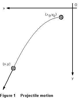
A projectile is an object which is falling freely under gravity, and at the same time undergoing horizontal motion. If gravity is indeed the only force on the object, its horizontal motion is unaccelerated. In that case, the equations of its motion are
![]() and
and ![]() (1)
(1)
 ...if its position
and velocity at time t = 0 are represented by (x0,y0)
and (v0x,v0y), respectively. Suppose now that
the coordinates of the projectile are measured at regularly spaced
times t = 0, T, 2T, 3T,. . Then we can use
the method of differences to determine its velocity and acceleration.
(The same method was used by the computer in the experiment titled "Falling
Bodies." Here we lay out "by hand" what the computer does
for you there.)
From Equations (1), the coordinates (x1,y1), (x2,y2), etc., are given by
![]()
and ![]()
for ![]() (2)
(2)
Now calculate the differences between successive values:
![]() , a constant
, a constant
and ![]() for
for ![]() (3)
(3)
Finally, the differences between successive differences, the second-order differences, of the values are given by
![]()
and ![]() for
for ![]() (4)
(4)
From Equation (3), if the horizontal motion is at constant velocity,
the first-order differences in x should be constant, and equal to
v0xT; and from Equation (4), if the vertical motion is
uniformly accelerated, the second-order differences in y
are constant and equal to gT2. Of course, even if (1)
is the correct description of the projectile's motion, your experimental
differences won't be exactly constant,  because
of experimental errors.
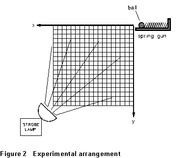
In the experiment, a steel ball is fired horizontally with an unknown velocity. A series of photographs of the ball in flight are taken at known time intervals. The superposition of a rectangular grid on the photograph allows x and y coordinates to be measured directly from the photograph. The initial velocity and the acceleration of the ball will be determined, respectively, from the first-order differences in x and the second-order differences in y.
(1) The steel ball is fired horizontally by means of a spring gun. A strobe light illuminates the ball very briefly each time it flashes, and the ball's position is recorded on the film. You should find the camera mounted in the proper position for taking the picture; try not to disturb its position as you use it.
(2) Fully cock the spring gun, and put the ball in the indentation nearest the left edge of the gun platform. The string that triggers the spring gun should run over the pulley that is mounted about a foot and a half from the gun. Slide the rectangular grid all the way to the left (out of the picture), so that the trajectory of the ball will be photographed against the plain black backcloth.
(3) Check the camera settings. It should be in good focus, the lens opening set to f/3.8, and the exposure time set at 1 sec (this is long enough to hold the shutter open through the entire flight of the ball).
(4) The Wavetek oscillator triggers the strobe light(s), and the Hewlett-Packard counter-timer reads its period (time between flashes, in milliseconds). Turn on the oscillator and set it for a strobe period of 0.020 to 0.025 seconds. Record the period. Position yourself so that you can operate the camera shutter (the red button labeled "2") with your left hand, and the string which fires the projectile with your right hand, at the same time. Have your lab partner turn out the room lights.
(5) Press the red shutter button and, as soon as you hear the camera shutter release, immediately pull the string to release the spring gun.
(6) Have your partner turn on the room lights, and turn off the strobe lamps. Reset the exposure time on the camera to 60 (that is, 1/60 sec), and the lens opening to f/11. Slide the rectangular grid all the way to the right so that it is in front of the camera. Cock the camera.
(7) Press the red shutter button (2). This reexposes the film, superimposing an image of the grid on your multiflash photograph of the ball in flight.
(8) Remove the exposed picture from the camera; your instructor will have shown you the right way to do this. It's important to pull the exposed film straight out of the camera so that it doesn't catch on any part of the camera. Allow the film to process itself for about 30 seconds after removing it from the camera, and then peel off the print.
(9) Your picture is a satisfactory one if it shows 10-15 clearly defined images of the ball, the grid is in focus, and the contrast is good enough to let you determine positions fairly readily. Tape your picture into your laboratory notebook; it is your primary data from this experiment! Starting with the image of the ball nearest the "gun," label the successive images on your picture 0, 1, 2, 3, . . .
(10) Pick a convenient point on the grid as your origin, and record the x and y coordinates of the center of each image of the ball. (You may find it helpful to use a magnifier to look at the picture. Grid lines are 1 cm apart, with every 10th one dark. The origin should probably be taken at one of the dark intersections. The directions of the coordinate axes shown in Figure 1 will be convenient.) Have your partner make an independent determination of these positions, and use the average of your two measurements in your calculations.
Complete steps 1-4 before leaving lab.
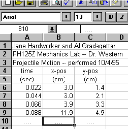
(1) Enter your t, x, and y data into a Excel spreadsheet. Use the first five rows of the spreadsheet for labeling as follows:
ROW 1: Your name and your lab partner's name
ROW 2: Course name and number and your lab instructor's name
ROW 3: Name of laboratory and date performed
ROW 4: Data labels for each column
ROW 5: Unit labels for each column
Place time values in column A starting at row 6. (HINT: you can use the FILL command to do this quickly.) Type your x data in column B starting at row 6. Type your y data in column C starting at row 6. Your spreadsheet should look something like this (if your flash period were 0.022 s):
 (2) Create an
"XY" graph with time values along the horizontal axis and x-position
data as the first dependent variable. [Note you must select "XY"
"Scatter" as the graph type!] Customize this graph so
that the data is shown with SYMBOLS ONLY (no lines). Title the graph and
label the axes appropriately.
(3) Use the spreadsheet's regression analysis capability to find the slope of the best straight line through the x-t data. In Excel, this is a function; if you had 10 data points in all, the call would be
=SLOPE(B6-B15,A6-A15)
(note the order of the variables). Put this call in cell E1, say; put a corresponding call of the function INTERCEPT, which returns the y-intercept of the straight-line fit, in E2. Cf Eq.(1): the slope and intercept are (respectively) v0x, the ball's initial horizontal velocity, and x0. (Excel has other functions providing statistical information about the fit. In particular, LINEST returns a complete statistical analysis, errors in coefficients, etc.)
(4) To see how well the least-squares straight line fits your data, plot this line along with the data. The equation has the form y = mx + b. In cell D6, put the formula
=$E$1*A6+$E$2
and use the FILL handle to copy this into the D column cells corresponding to your data values. (Notice when the formula is copied that the cell addresses $E$1 and $E$2 don't change. These cells are said to be "anchored;" that's what the dollar signs do.) Put a title for the column, such as "x(fit)", in D4. These are the values of x(t) calculated from your best-fit line.
Use the spreadsheet to make a graph showing x (data) and x (fit) vs. t. In Excel, the Chart Wizard will lead you through this. Include a printout of this graph in your lab report. Also include a copy of the QUATTRO regression output.
(5) We now wish to find the acceleration of gravity using a similar process. Y vs. t is not a linear dependence, but vy is. So we will need velocity data for the projectile's vertical motion. We will put this data in COLUMN E. In CELL E7 (yes, E7, not E6) put the formula
=(C8-C6)/(A8-A6)
As you can see, this is the average velocity over the first two time intervals. In the case of constant acceleration, the average velocity for any time interval is the instantaneous velocity at the midpoint in time [PROVE THIS ASSERTION IN YOUR LAB REPORT], hence we place this value in E7, to correspond to the time in A7.
Fill this formula into the remaining cells in column E, stopping one short of the number of original data points. You now have vertical velocity vs. time data. Plot this data as you did the x-position data (but on a different graph). Do a least-squares regression and find the acceleration of gravity. Plot your least-squares line on the velocity graph as you did in the case of the x-position data. Include a copy of this graph in your report and quote the acceleration of gravity. (What is the "y-intercept" of this graph?) Remember to save this graph.
(6) Finally make a third graph, this time of y vs. x (x is the independent variable). By eliminating t between the expression for x and the expression for y in Eq. (1) above, you can write an equation for y as a function of x. All quantities (g, v0y, v0x, x0, y0) are known from your analysis. Make an additional column of calculated y values based upon the formula you derive, and the best fit parameters you have deduced. Plot values obtained from this formula along with you data. [Remember: data with SYMBOLS, no lines, and formula values with LINES, no symbols. Include this graph with your report and comment about the agreement between data and formula based upon best-fit parameters.]
Report your best overall values for the initial velocity of the ball (v0) and the acceleration due to gravity (g), with estimates of the experimental uncertainty in these values.
last update 6/96