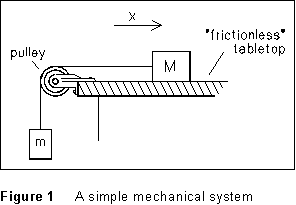
 Figure 1 shows
a very simple mechanical system which we are going to examine from the
point of view of Newton's second law of motion:
Figure 1 shows
a very simple mechanical system which we are going to examine from the
point of view of Newton's second law of motion:| Table of Contents |
Crummett and Western, Physics: Models and Applications,
Sec. 5-2,3,4
Halliday, Resnick, and Walker, Fundamentals of Physics (5th
ed.), Sec. 5-3 to 5-6
Tipler, Physics for Scientists and Engineers (3rd ed.), Sec.
4-2,3
 Figure 1 shows
a very simple mechanical system which we are going to examine from the
point of view of Newton's second law of motion:
![]() (1)
(1)
where F is the resultant (the vector sum) of all the forces that act on the object of mass m, and a is its acceleration. Consider the very simple system sketched in Figure 1. There is a block of mass M resting on a frictionless horizontal surface. It is connected to another hanging mass m by a string which passes over a massless, frictionless pulley. (This is clearly an idealized situation!) Since the pull of the string is the only horizontal force that acts on M, it is clear that the system will accelerate.
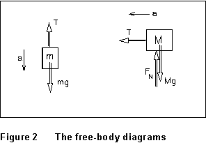 Free-body
diagrams for the two masses in Fig. 1 are shown in Figure 2. In each,
the body is isolated and all the forces which act on it are indicated.
FN is the normal support force of the table top,
and T the tension in the string connecting the two masses.
Equation (1) applied to these two diagrams gives
![]()
and ![]()
If we eliminate T between these two equations, we are left with
 (2)
(2)
In this experiment, you'll set up a situation closely equivalent to that of Figure 1, using a linear air track to approximate a frictionless surface; determine the acceleration experimentally and compare it to Equation (2); and try to infer the reasons for any differences you may observe between the experimental situation and the analysis given above.
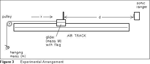
The translation of Figure 1 into the laboratory is sketched in Figure 3 above. Note: Before beginning this experiment, you should already have completed the orientation exercise on the Sonic Ranger and the PC which appears at the beginning of this chapter.
(1) In this laboratory you will be recording the position of an air-track glider using the sonic ranger. Position the sonic ranger about 30 cm beyond the end of the air track nearest the wall. Put a glider on the air track, turn on the blower (air output at position 3), and collect data with the SR. Adjust the SR until it can reliably "see" the glider at all points along the length of the track. If you can't get the SR to see the glider all the way to the far end after a few minutes of adjustment ask your instructor for advice. (Actually it's all right if the SR loses the glider when it is close, say within 30-40 cm of the SR end of the track.)
Level the track by adjusting the screws in the feet of the track. Ideally the glider will remain stationary when placed at any point on the track. In fact, you may find subtle dips or humps in the track. Do the best you can.
(2) Record the ambient temperature (there is a thermometer on the wall of the laboratory) and calibrate the sonic ranger.
(3) Give the glider a gentle push down the track and record a set of position vs. time data. Save this data to disk. Later you will use this data set to determine how precisely level the track is.
(4) You are now ready to collect data for accelerated motion. Measure the mass of your glider (leave the string attached) and the masses of any weights you will use for m. Attach a thread to the hanger, run the thread over the pulley at the end of the track, and hang a small hanger on the end. Your goal is to measure the acceleration of the glider with five or six different values of mass (m) hanging on the end of the string, and to compare the results to Eq.(2). The mass values should range from roughly 5 g to at least 30 g or more, depending on what masses are available; in roughly equal steps.
(5) Choose one of the masses you are going to use -- preferably neither the biggest nor the smallest. Hang the mass on the end of the string. Place the glider at the end of the track farthest from the SR.
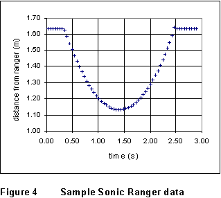 Start the data collection
and then gently push the glider toward the SR. Check the collected
data to insure that it looks clean and reasonable. You should see a parabolic
"U" shape, as in Fig. 3. In Fig.3, the experimenter caught the
glider at t = 2.50 sec; if not, the graph would show cusps where
the returning glider strikes the bumper and rebounds.
(6) When you have data you consider satisfactory, save the data to disk.
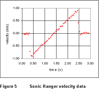
(7) The object of the game, remember, is to get a value for the acceleration of the glider. Obtain a value for the acceleration from the x-t graph and a second from the v-t graph. The v-t graph for the data of Fig.4 is shown as Fig.5. They should agree!
(8) Repeat the acceleration measurements of (5) - (7) above four more times for the same mass value -- five runs altogether for this mass value.
 (9) Repeat
the acceleration measurements of (5) - (7) above for four or five other
mass values on the end of the string. Don't repeat (8) -- that is, just
do one run of each of these mass values.
(1) First examine your first run, the unweighted glider on the level track. Transport your data into a spreadsheet, and use the linear regression functions (SLOPE, INTERCEPT) to do a best-straight-line fit to the v vs. t data. The slope of the best-fit line produced by the fit is the acceleration of the glider. Quote this result, with error. For a perfectly straight, level track, it should be zero. If this acceleration is greater than 0.01 m/s2, you will need to subtract this value from all subsequent calculated accelerations.
(2) Next consider the five runs you made for the first mass value. You got ten measurements of the acceleration from fitting them "manually"; calculate the mean, standard deviation, and standard error of the acceleration from these ten values.
(3) Now transport one or more of these data sets into your spreadsheet program, and use the linear regression tools to do a best-straight-line fit to the v-t data and get a value for the acceleration. How do these values of a compare to the result from the manual fits? Are they in agreement, within experimental error? The point here is to investigate how good the manual fitting procedure is. Your writeup should include graphs of v vs. t and x vs. t for at least one of these runs, including both data and curves representing the best fit.
(4) Finally, consider the data sets in which you measured accelerations for different masses. Use these (including the one you repeated several times) to produce a graph of Eq. (2). Use your best values of acceleration for the vertical axis and m/(M+m) values for the horizontal axis. Note that you can correct for the 9.0 g mass of the pulley by adding 4.5 g to the mass of the glider. (The reason for the factor of 2 will become clear later in your mechanics course, when you study rotational motion.)
Perform a least-squares fit to the graph you have made. Plot the best- fit straight line (lines, no symbols) along with the data (symbols, no lines). Compare the slope obtained to the theoretical value implied by Eq. (2), and comment regarding agreement and uncertainties.
Conservation of Mechanical Energy
last update 6/96