 Crummett and
Western, Physics: Models and Applications, Sections 8-2,3,
14-3
Crummett and
Western, Physics: Models and Applications, Sections 8-2,3,
14-3Halliday, Resnick, and Walker Fundamentals of Physics (5th ed.), Sections 8-7, 16-6
Tipler, Physics for Scientists and Engineers (3rd ed.), Sections 6-5,6, 12-5
| Table of Contents |
Crummett and
Western, Physics: Models and Applications, Sections 8-2,3,
14-3
Halliday, Resnick, and Walker Fundamentals of Physics (5th
ed.), Sections 8-7, 16-6
Tipler, Physics for Scientists and Engineers (3rd ed.), Sections
6-5,6, 12-5
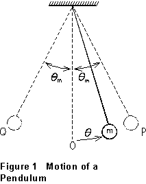
A simple pendulum consists of a small mass suspended from a fixed point
by a light string, free to swing back and forth under gravity. In Figure
1, the object m was released from point P, at which the string makes
an angle ![]() with the
vertical. If the friction of the air, and at the suspension point, can
be neglected, the total mechanical energy of the system will be constant.
The tension in the string does no work on m, so the potential energy
is just that due to gravity, and
with the
vertical. If the friction of the air, and at the suspension point, can
be neglected, the total mechanical energy of the system will be constant.
The tension in the string does no work on m, so the potential energy
is just that due to gravity, and
![]() (1)
(1)
At either end of the swing, ![]() and
v = 0, so
and
v = 0, so
![]()
Eliminating E and solving for v gives
![]() (2)
(2)
The velocity of mass m at the bottom of the pendulum's
swing (![]() ) is therefore
) is therefore
![]() (3)
(3)
Now let's calculate the period of the pendulum from this. In a time
dt the distance that the mass moves is v dt. The angle through
which the pendulum swings in this time is ![]() ,
so
,
so
![]()
Rearranging this and integrating it, we can find the time the pendulum takes to swing from O to Q:
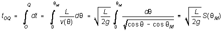
and since this is one quarter of the complete cycle, the period of the pendulum is
![]()
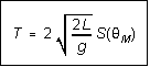 (4)
(4)
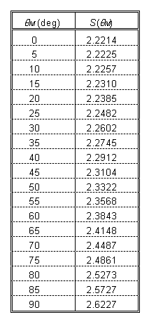 The integral
 ![]() that
appears in (4) cannot be carried out in simple closed form (except in the
limit of very small
that
appears in (4) cannot be carried out in simple closed form (except in the
limit of very small ![]() ,
in which case
,
in which case ![]() ).
It is one of a class known to mathematicians as elliptic integrals.
For any given
).
It is one of a class known to mathematicians as elliptic integrals.
For any given ![]() ,
however,
,
however, ![]() can be
evaluated (to any degree of precision you like) by numerical integration.
A table of
can be
evaluated (to any degree of precision you like) by numerical integration.
A table of ![]() is given
at right, for values of
is given
at right, for values of ![]() in
5-degree steps.
in
5-degree steps.
In this experiment, you will create a simple pendulum with a loop of thread and a mass; investigate the effect of the pendulum's amplitude on its period of oscillation; determine the acceleration of the pendulum near its turning points; determine its maximum angular velocity; and save data files for further analysis.
First, some general remarks about the shaft encoder. This laboratory uses these devices to generate angular displacement data as a function of time. A shaft encoder is basically just a wheel with N equally spaced holes near its perimeter (the ones we use here have N = 512). They have two detectors, spaced about 1/4 of a hole diameter apart, to tell whether a hole is next to a detector or not. Each detector puts out a digital "1" or "0" depending on whether there is a hole; using two detectors lets the software tell which way the shaft is turning. The associated computer software will provide graphs of angle (in radians) vs. time and of angular velocity vs. time are available. Data can be edited, and saved to a file; these files can be imported by Excel or other spreadsheet software for further analysis.
(1) Make your pendulum just by hanging one big loop of thread over the pulley, and fastening a mass on the other end. The shaft friction is so low that the loop will not slip on the pulley. Use a hex nut for your pendulum mass; you can attach it to the intact loop just by looping through the hole in the middle and around. The pendulum length should be something like 0.50 - 0.70 m.
(2) Measure the mass of the nut (your pendulum bob) on the pan balance. Carefully measure the length of the pendulum, from the axis of the pulley to the center of mass of the nut. Make clear in your lab notebook how you do this. Carry out several trials of this measurement, and calculate the mean and standard error of L.
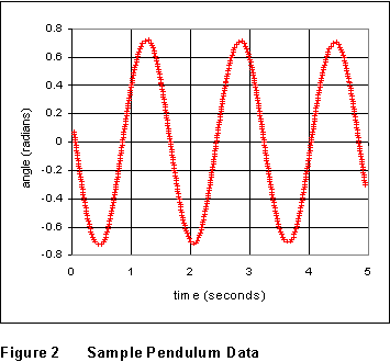
(3) Set the program so that it will take data for several complete cycles and displays 100 or so data points per cycle. Release the pendulum from an initial angle of around 30 degrees, and acquire a data set. A sample set of data is shown in Figure 2 at the right. Save your data to a file, and record the filename in your lab notebook.
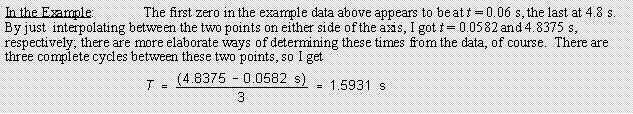
(4) For this first data set, measure and record the period of the pendulum from the graphed data, as precisely as you can. There are various ways you can do this, one of which is illustrated in the box below, for the data of Figure 2; but in your lab book, explain clearly what you did to measure the period.
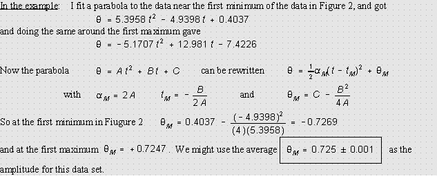
(5) Likewise, there are several ways you can measure the amplitude
of the pendulum's motion. You can read the lowest and highest single data
values directly from the graph of your data. Perhaps a better way (since
it uses a number of data values, rather than one) is to clip out a small
section of the data near an extremum, fit a parabola to these points, and
calculate the peak value of the parabola. (![]() for the pendulum isn't parabolic, of course; what you're doing is to find
the parabola that, at the peak, has the same peak height, curvature,
etc. as does the data.) In any case, again, measure and record the amplitude
and explain clearly how you determined it.
for the pendulum isn't parabolic, of course; what you're doing is to find
the parabola that, at the peak, has the same peak height, curvature,
etc. as does the data.) In any case, again, measure and record the amplitude
and explain clearly how you determined it.
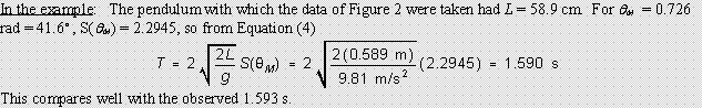
(6) Check your procedures before going further, by calculating
T from Equation (4) using your measured values of L and ![]() ,
and comparing it to your measured value of T. The agreement should
be quite good.
,
and comparing it to your measured value of T. The agreement should
be quite good.
(7) Take several (four to eight) more data sets, varying the
release angle between about 10 degrees and about 60 degrees. Save all your
data sets to disk. You needn't be very precise about measuring the "lanch
angle," as you infer ![]() from
your data sets, as above. Also, for each of your data sets, determine the
peak value
from
your data sets, as above. Also, for each of your data sets, determine the
peak value ![]() of the
angular velocity vs. time graph. (Note: fitting the
peaks in your data to get
of the
angular velocity vs. time graph. (Note: fitting the
peaks in your data to get ![]() and
and
![]() can either be done
by "eyeball" in the lab, or later using a spreadsheet such as
EXCEL, whichever you find convenient. The former is quicker, the latter
more precise.)
can either be done
by "eyeball" in the lab, or later using a spreadsheet such as
EXCEL, whichever you find convenient. The former is quicker, the latter
more precise.)
(8) For at least one of your data sets, you will want
to have measured the angular amplitude (![]() )
at every maximum and minimum.
)
at every maximum and minimum.
(1) For at least one of your data sets, include in your lab notebook book the actual graphs of the angle vs. t and angular velocity vs. t data.
(2) Measure and record the amplitude of the pendulum for each of your data sets. Compare the dependence of the period of the pendulum on its amplitude, as you have measured them, with the theory developed above in the Introduction.
(3) The maximum kinetic energy of the pendulum occurs when the mass is at the bottom of its arc:
![]() (5)
(5)
while the potential energy is maximum at the turning points:
![]() (6)
(6)
If the total mechanical energy is conserved,
![]() (7)
(7)
Make a table showing UMAX, KMAX, and E for each of your data sets. Do your data support the theorem of conservation of mechanical energy?
(4) In procedure (8) you measured the angular amplitude at several different times for one of your data sets. You may observe that the amplitude decreases slightly with time; this is because there is some slight energy loss due to frictional forces in the system. Use your data to give a value for the rate of energy loss, expressed as, say, % of total energy lost per cycle.
last update 7/97