Chapter 3: Mechanics Experiments
Familiarization with Position, Velocity, and Acceleration Measurement
References
Crummett and Western, Physics: Models and Applications, Sections
3-1, 3-2, 3-5
Halliday and Resnick, Fundamentals of Physics (4th ed.), Sections
2-2 to 2-5
Tipler, Physics for Scientists and Engineers (3rd ed.), Chapter
2
This orientation is designed just to familiarize you with the apparatus
that you'll use throughout this laboratory.
Introduction
Much of the data that you take in this laboratory will be acquired using
your laptop computer in conjunction with some simple external devices controlled
by homemade software:
- The laptop computer acts as a stopwatch, scratchpad,
and data display and analysis tool.
- The BIB box plugs into your computer's printer port,
and allows the computer to control the shaft encoder and sonic ranger as
well as other devices.
- The sonic ranger is a poor man's sonar, emitting ultrasonic
"pings" and timing their echoes.
- The shaft encoder is a "smart" pulley that
can keep track of its angle of orientation.
- Numerous analog devices whose output voltages are read by an A/D converter
in the BIB box.
In this exercise you will use your laptop computer, the BIB box, and
the sonic ranger to gain some familiarity with the software and equipment
as well as obtain position, velocity, and acceleration measurements. As
you go through this exercise, keep notes in your laboratory notebook of
what you do and what you observe, record all your results, etc. Your instructor
may want to collect your notebooks and look over your work, but probably
will not grade it. OK, let's get started.
Data Acquisition Software
The first thing you need to do is get a copy of the data acquisition
software. There are two ways to do this. You may either (1) transfer the
software to your computer over the Internet, or (2) your instructor may
provide the software on a floppy disk. If you wish to transfer the software
over the net, log on to the network and bring up Netscape. Go to the site
http://www.Rose-Hulman.edu/~hatten/index.html
 From this page
you will be able to call down the physics lab software in the form of a
"zip" file called "physics_lab_software.zip". A zip
file is a compressed data file written by the WinZip program. A zip file
may contain many files compressed into one. Save this zip file to your
hard drive. It might be a good idea to make a new directory to hold it.
Then double click on the zip filename in the Windows Explorer. The WinZip
window (shown at right) will open up. Click on the Extract button, and
give the path to where you want the files. Once the files are extracted,
you may delete the "physics_lab_software.zip" file to save hard
drive space.
From this page
you will be able to call down the physics lab software in the form of a
"zip" file called "physics_lab_software.zip". A zip
file is a compressed data file written by the WinZip program. A zip file
may contain many files compressed into one. Save this zip file to your
hard drive. It might be a good idea to make a new directory to hold it.
Then double click on the zip filename in the Windows Explorer. The WinZip
window (shown at right) will open up. Click on the Extract button, and
give the path to where you want the files. Once the files are extracted,
you may delete the "physics_lab_software.zip" file to save hard
drive space.
If your instructor wishes, or if the network is down, the physics_lab_software.zip
file will be available on floppy disk. Copy the zip file to a directory
on your hard disk, and extract the software in the same manner as described
above.
Data Acquisition Hardware


Now that you have the software, let's move on to the hardware. The various
data acquisition devices we will use all go through the BIB Box (See Figure
2) to talk to your computer. Plug the BIB Box's A/C adapter into one of
the power outlets on your lab table. Plug the adapter cable into the BIB
Box. Connect the BIB Box data cable to the printer port on the back of
your laptop. The first device we will be using is the sonic ranger (See
Figure 3). Plug the cable from the sonic ranger into the BIB Box. You will
need a short adapter cable (~ 5 inches) to make this connection.
Now run the program called "Lab Startup.exe." This program
is the shell program which allows you to select the instrument that you
will be using. Select the Sonic Ranger Software option and click OK. The
sonic ranger program will come up (See Figure 4). Note that the program
has both a button bar and pull-down menus. The button bar gives you fast
access to frequently-used commands. All of these commands  may
also be accessed through the pull-down menus. In addition, the pull-down
menus have additional commands not found on the button bar. The software
uses the standard Windows 95 file manipulation commands and windows. Move
the mouse over the items on the button bar. The title of the command will
pop up under each button as the mouse passes over it. Browse through the
pull down menus and familiarize yourself with which commands are where.
Some of them may not yet make sense to you, but they will soon.
may
also be accessed through the pull-down menus. In addition, the pull-down
menus have additional commands not found on the button bar. The software
uses the standard Windows 95 file manipulation commands and windows. Move
the mouse over the items on the button bar. The title of the command will
pop up under each button as the mouse passes over it. Browse through the
pull down menus and familiarize yourself with which commands are where.
Some of them may not yet make sense to you, but they will soon.
Now let's take some data with the sonic ranger. Click on the "set
parameters" button on the button bar to set your data acquisition
parameters. The parameters window will open up allowing you to input the
room temperature, set the frequency with which the ranger sends out pulses,
and set the total number of data points taken. The room temperature is
available from the thermometer on the wall in the front of the room in
the labs. Set the ping rate at 75 Hz and the number of data points at 200.
Then click on OK. You are now ready to take position vs. time data with
the ranger. Hold your hand in front of the ranger (at least 40 cm away
from it). Click on the "take data" button, and move your hand
back and forth. A position vs. Time graph will appear on the screen with
a plot of your hand's position on it. The plot should look something like
Figure 5. The software allows you to do numerous things with this plot
such as zoom in on a particular range, fit a line or parabola to sections
of the plot, remove bad data points, extract the coordinates of a point
on the plot, or dump the plot to a printer.
Let's try a few of these. Click on the "zoom" button on the
button bar. This enables the zooming function. Move the mouse to the upper
left hand corner of a region you would like to zoom in on. Left click and
drag the mouse down and to the right.  An
expanding rectangular box will appear indicating the region you have selected
to zoom in on. When you have selected the region you want, release the
mouse button. You should now be looking at an expanded plot of the selected
region. If you are unhappy with the region you selected, you can click
on the "zoom out" button and start over. Now let's try a parabola
fit of the zoomed region. Click on the "plot quadratic" button.
An
expanding rectangular box will appear indicating the region you have selected
to zoom in on. When you have selected the region you want, release the
mouse button. You should now be looking at an expanded plot of the selected
region. If you are unhappy with the region you selected, you can click
on the "zoom out" button and start over. Now let's try a parabola
fit of the zoomed region. Click on the "plot quadratic" button.
The program is now ready to let you do an eyeball fit of a parabola
(quadratic) to the data. Since three points determine the equation of a
parabola uniquely, you will left click at three points on your plot where
you envision a parabola passing through. (You don't have to click on actual
data points.) After you have clicked three times, a parabola and its equation
will appear on the graph. Continued left-clicking will re-adjust the positions
of the first, second, and third points in a revolving sequence. Try it
and see if you follow what's going on. Your eye is a pretty good judge
of whether you have the curve in the right place. Readjust the coordinates
of the three points until you think you have the best fit of your data.
Then ask your instructor or lab assistant to take a look at it (See Figure
6). If you wish to start all over on your fit, you can click on the "clear
points" button which will remove the three marked points, the parabola,
and its equation. You may now start over again by clicking on the "plot
quadratic" button. Do this and let your partner re-do the fit. When
you are done with the fit, you can view the entire plot again by clicking
on the "zoom out" button. Do so now. You should be looking at
the entire plot once more.
If you wish to know the coordinates of a particular data point (or any
point on the graph for that matter), you can find these using the "point
coordinates" command under the "left-click" pull down menu.
Then when you click somewhere on the screen, the coordinates of where you
clicked appear on the screen. Try this now. This feature is very useful
for measuring time and position differences from the graph.
 Try several
other objects as targets, as well as your hand. Move the targets toward
and away from the Sonic Ranger. Try a flat target like a book, and a skinnier
one, like the edge of a book. Record all your observations on this
in your lab notebook. Are echoes equally smooth for all kinds of
targets, or does data "jump around" more for some targets than
for others? What is the best target for work in the two-to-four foot range?
Lower the ping rate and try some targets in the six-foot to ten- foot range
(the floor tiles are a handy way of estimating horizontal distance, once
you know their dimensions).
Try several
other objects as targets, as well as your hand. Move the targets toward
and away from the Sonic Ranger. Try a flat target like a book, and a skinnier
one, like the edge of a book. Record all your observations on this
in your lab notebook. Are echoes equally smooth for all kinds of
targets, or does data "jump around" more for some targets than
for others? What is the best target for work in the two-to-four foot range?
Lower the ping rate and try some targets in the six-foot to ten- foot range
(the floor tiles are a handy way of estimating horizontal distance, once
you know their dimensions).
Use one of your rocky data sets to try the "deletion" functions
under the "Left-click" pull down menu. Under this submenu there
are two items: (1) "delete point" which excises bad data points
from the data set, and (2) "replace point" which replaces bad
data points with a linearly extrapolated value based on the points immediately
before it and after it in the data set. Try cleaning up some of the bad
data points in your data set. When do you suppose these functions are useful?
Velocity and Acceleration Plots
Take a set of data on a moving target. A data set contains just t and
x values, and the software displays a position vs. time plot by default.
The software can also display the corresponding velocity vs. time and acceleration
vs. time plots. This is accomplished by clicking on the velocity or acceleration
plot buttons on the button bar. Give this a try. The software computes
velocity and acceleration from the position data by simple difference formulas
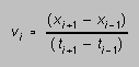 and
and  (1)
(1)
for the various displays. You will notice that the velocity and acceleration
plots are not as "nice" and the position plot. This is an inevitable
result of the use of the above difference formulas, which are approximations.
Small errors get amplified when these formulas are used.
Saving and Transferring Data
The software automatically saves the position data to a default file
every time you take a new data set. The default file name is "erase.me"
and it is saved to the same directory where your data acquisition software
is located. The purpose of this default data file is to prevent data loss
in the event of computer lockup or network problems prior to intentionally
saving the data. Be aware that this backup copy of your data is there in
the event of a problem. Also be aware that the next time you take data,
the default file will be overwritten with the new data set.
When you get a data set you wish to keep, you may save the data to a
file name of your own choosing using the File|Save or File|Save
As options from the pull down menu, or clicking on the file save icon
on the button bar similar to any other Windows 95 program. As an exercise,
create a small (50 data points) data file, and send it to your F: drive
on the server.
You will notice that files are saved with a default extension of ".xls"
which is normally indicative of a Microsoft Excel file. The files that
the data acquisition software saves are not in the Excel format, but may
be opened in Excel using the File|Open commands. The data files are formatted
so that they will parse correctly into columns in Excel. Excel may then
be used for more extensive analysis/graphing of the data.
Studying position, velocity, and acceleration.
(a) As a warm-up, predict what the graphs of x vs. t and
v vs. t will look like for a stationary object, and
make small sketches in your notebook. When that is done, take some data
for a stationary object (like a wall or a chair), and check that the graphs
in the computer are similar to the ones that you drew.
You have probably noticed that there is often some "jitter"
in the (x-t) data, and that this produces glitches in the (v-t)
graph which are sometimes fairly wicked. Some of the jitter is due to software
timing, and some of the jitter is due to irregular returning echoes from
the target. Another complication which will also show up is that your pinger
may pick up sounds from other pingers - and this WILL mess
up your data.
The velocity and acceleration points are calculated using very simple
difference routines (Equations (1) above). We wind up with two fewer velocity
values than positions, and fewer acceleration values than velocity values.)
When data is saved to a file, only the x vs. t data is saved. The
computer's (v-t) and (a-t) graphs are just to give you an
idea of what's going on, with minimal processing.
(b) The graph of velocity vs. time for constant-velocity motion is a
straight horizontal line. For this very simple motion, make a small sketch
in your notebook of what you expect for the graph of x vs. t. Now
move your hand or other target at what you think is constant velocity until
you get some reasonable-looking data. Figure out a way to determine the
velocity from this graph. You can use simple multiplying and dividing as
a check on what the Line function gives you.
Plot the (v-t) graph on the screen. The velocity values should
fall in the same general range you got before. (Do they?)
Now try making a graph that shows motion with constant velocity with
a reversal of direction -- the (x-t) graph would look something
like Figure 2, below. Work on this until you get the constant-velocity
sections pretty straight and the reversal (the "corner") pretty
sharp. Try to get about the same velocity coming and going.
For this motion, what should a graph of v(t) look like? Make
a small sketch of the anticipated (v-t) graph in your lab
notebook before you begin. Take data until it looks about right in x
vs. t. Then see if the (v-t) graph also looks like what you
expected. What do you think the acceleration vs. time graph will
look like? Take a look at it! Record your observations and conclusions.
Shown in Fig. 3 is a different motion, this one on a graph of velocity
vs. time. Try to generate a sonic ranger graph of v vs. t which
looks like it. Before you start out, make a small sketch in your lab notebook
of what you think the (x-t) graph for this case should look like.
Take the minimum velocity to be zero.


(c) In this part you will try to make a target move with a small constant
(1 or 2 m/s2) acceleration. Before you generate any data, make
a small sketch of what you think the x vs. t, v vs. t, and
a vs. t graphs will look like. Then go ahead and try your hand at
it.
When you get some (x-t) data which looks reasonable to you, try
to determine the value of the acceleration. Try to get a value from the
(x-t) graph (helped by curve fitting), from the (v-t) graph
(with or without curve fitting) and -- if possible -- the (a-t)
graph. Record your observations and conclusions.
Falling Bodies
last rev 9/97 - DLH