Chapter 3: Mechanics Experiments
Falling Bodies
References
Crummett and Western, Physics: Models and Applications,
Sections 3-2, 3, 5; 16-4, 5
Halliday, Resnick, and Walker Fundamentals of Physics (5th
ed.), Sections 2-4, 5; 6-3
Tipler, Physics for Scientists and Engineers (3rd ed.), Sections
2-4; 5-2; 11-4
Introduction
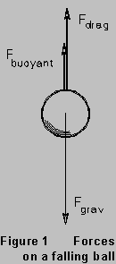 (In which it
is seen that free fall is not so simple as we thought it was.) Objects
falling "freely" in our everyday experience really aren't free;
there is always a "drag" force opposing the motion, and an upward
static "buoyant" force, both due to the air through which
the object moves. The buoyant force is equal to the weight of the displaced
air:
(In which it
is seen that free fall is not so simple as we thought it was.) Objects
falling "freely" in our everyday experience really aren't free;
there is always a "drag" force opposing the motion, and an upward
static "buoyant" force, both due to the air through which
the object moves. The buoyant force is equal to the weight of the displaced
air:
 (1)
(1)
where  is density.
( The density of air depends on local conditions, but is about 1.2 kg/m3.)
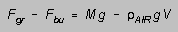
The net static downward force on the object, its "effective
weight", is
is density.
( The density of air depends on local conditions, but is about 1.2 kg/m3.)
The net static downward force on the object, its "effective
weight", is
 (2)
(2)
For convenience, let's call this force  ,
where the "effective mass"
,
where the "effective mass"
 (3)
(3)
MEFF, for example, and not M, is what you read
when you "weigh" the object on a pan balance. For a solid object
like a baseball,
and we will ignore the difference between MEFF and
M. Then in these terms, Newton's second law for the falling object
says that

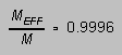
where FD is the drag force of the air. The drag force
on an object moving at speed v is given by
 (4)
(4)
where CD is a dimensionless constant called the "drag
coefficient" that has to do with the shape of the object; and A
is the object's "frontal" area. Then the acceleration of the
falling object is
 (5)
(5)
-- and we can start to see what will happen.
There are two limiting cases. (i) As the ball begins to fall,
its v = 0 and the second term in (5), due to the drag force, is
(for a time) negligibly small. The object then initially falls with a uniform
acceleration that is nearly equal to g. 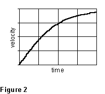 As
time passes, v increases, and according to (5) its acceleration
decreases. The speed of fall continues to increase, but at a diminishing
rate, as is seen in Figure 2. (ii) Eventually the object approaches a speed
at which the two terms of (5) are equal. At this speed the acceleration
goes to zero:
As
time passes, v increases, and according to (5) its acceleration
decreases. The speed of fall continues to increase, but at a diminishing
rate, as is seen in Figure 2. (ii) Eventually the object approaches a speed
at which the two terms of (5) are equal. At this speed the acceleration
goes to zero:

so the terminal speed of the falling object is
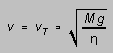 (6)
(6)
with 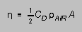
 has the
dimensions of 1/length, and you can think of
has the
dimensions of 1/length, and you can think of  as,
very roughly, how far the object must fall to approach terminal speed.
We suggest you look at two falling objects in this experiment: a soccer
ball and a very light object such as a paper coffee filter. The latter
is so light that it attains terminal speed by the time it has fallen 1
m or less; the ball, on the other hand, moves with essentially uniform
acceleration for its first few meters.
as,
very roughly, how far the object must fall to approach terminal speed.
We suggest you look at two falling objects in this experiment: a soccer
ball and a very light object such as a paper coffee filter. The latter
is so light that it attains terminal speed by the time it has fallen 1
m or less; the ball, on the other hand, moves with essentially uniform
acceleration for its first few meters.
Equipment
Sonic Ranger, BIB box
Laptop computer (yours) running kinematics software
ball, coffee filters or other low-mass specimen
meter stick, balance
Procedure
(1) Some time during the lab period, use the balance to determine the
mass of the ball and coffee filters. Be sure to zero the balance carefully
before beginning; this is done by rotating the black thumb-sized object
at the lower left front of the balance. Each partner should make at least
one independent measurement of each mass. Estimate the experimental
uncertainty in the measurement.
(2) Some time during the lab period, make a careful measurement of the
diameter of your ball. You'll have to come up with your own method, using
meter sticks, books, walls, etc., etc. Describe your method clearly in
your lab notebook. Repeat the process several times, and calculate the
average value and its standard error.
The order in which you investigate your two freely falling objects isn't
important: you can take ball data first, or last. There aren't enough balls
for everyone to work in the same order.
The computer software acquires (x vs. t) data for the falling
object, at regular time intervals. From this you can get a graph of the
(x,t) data, as well as (v,t) and (a,t) plots derived
from the (x,t) data. You can also fit a line or parabola to your
data if you desire. When you do a fit to a data set, record the equation
of the fit in your lab notebook, and note the data file name or trial with
which the fit is associated.
The Falling Ball
The ball is heavy enough so that in falling a meter or so it is very
much less affected by air drag; the motion you expect to see is essentially
free fall.
(3) Practice dropping the ball below the sonic ranger. Note that you
should have a minimum distance of about 0.4 m between the ball and the
ranger. You may find that the data gets "noisy" as the distance
from the ranger increases; if so, try changing the pinging frequency from
the default value set by the program. Always start the pinger before
releasing the ball, so that the data set you gather begins with the object
at rest. When you have dropped-ball data that looks good, determine the
acceleration of the falling ball from the (x,t) graph.
(4) Now look at the (v,t) graph of these same data, and determine
the acceleration. Describe how well you think the curve matches the points
(these aren't data points; they're derived, by the software, from the x-t
data by an average-velocity procedure.) Save this data set to a file.
(5) Now repeat steps (3) and (4) to obtain a second set of data, and
repeat the analysis above to determine the acceleration of the falling
ball. If one partner took the lead in analyzing the first set of data,
then the other partner should take the lead in analyzing this second set.
Make it clear in your account in your lab partner who did what, and to
which. Save this data set to a file.
Coffee Filters
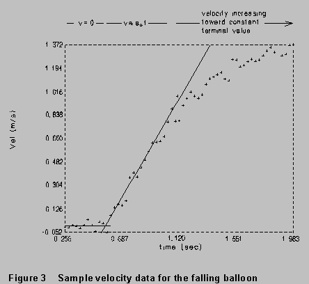
Here we have you drop an object of very low mass, which attains terminal
speed very quickly. Velocity data from a fairly typical example are shown
in Figure 3. Although this object does not quite reach its terminal speed
in the time shown here, the behavior described above is evident: decreasing
initial acceleration, approaching a constant speed. Note the initial
constant acceleration is not equal to g.
 (6) Start with
three nested filters and proceed as you did for the ball, and practice
until you get data that look clean to you. When you do, estimate the terminal
speed vT from the (x,t) graph. You want to obtain
position vs. time data for the entire range of the coffee filters'
fall, from just before release until they reach terminal speed. You may
have to adjust parameters in the software to achieve this. Explain what
you did, and what value you got for vT, in your lab notebook.
(6) Start with
three nested filters and proceed as you did for the ball, and practice
until you get data that look clean to you. When you do, estimate the terminal
speed vT from the (x,t) graph. You want to obtain
position vs. time data for the entire range of the coffee filters'
fall, from just before release until they reach terminal speed. You may
have to adjust parameters in the software to achieve this. Explain what
you did, and what value you got for vT, in your lab notebook.
(7) Now go to the (v,t) graph, and from it obtain an estimate
for the terminal velocity vT . Explain what you did,
and what value you got for vT, in your lab notebook.
Save this data set to a file.
(8) Peel off one of the three filters. Repeat steps (6) and (7) using
two filters to obtain additional data, and determine the terminal speed,
interchanging the roles of lab partners as you carry out the measurements.
Peel off one more filter and repeat steps (6) and (7) using one filter.
Analysis
The Ball
The lab work with the sonic ranger has, in effect, provided you with
values of A, B, and C in the equation
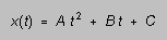 or
or  (7)
(7)
for each data set. Now, you are to check these values by fitting
each of your (x,t) data sets to the same function form in an Excel
spreadsheet.
To do this, first import the data into Excel. (You do this from File
Open, just as if you were opening a spreadsheet file; specify your
data file drive, type, and name in the Open dialogue box. Excel will bring
up a Text Wizard to do the translating.) Copy the "t"
column into another column, and set up the x(t) calculated from
Equation (7) in the column next to where you copied the "t"
data. Establish cells for the values of A, B, and C
so that you can adjust these quantities and see the graph change. Vary
these values until you think you have as good a fit as you can get to the
experimental x(t) data. Record the "best" A, B,
and C values for each set.
Include in your writeup a Excel graph which shows the experimental x(t)
data and also the curve calculated from your "best" values for
A, B, and C, for one of the data sets; and
another graph which shows the experimental v(t) and also the line calculated
from the same values of A and B. Make a statement in the
"conclusions" to your lab writeup as to how well the laboratory
values of A, B, and C compare to the spreadsheet values.
Indicate what you believe to be your overall best experimental value
for the acceleration of the falling ball. Estimate the experimental
uncertainty in this overall value, and describe how you arrived at this
estimate of error.
Based on what you know about drag and buoyant forces, what should the
acceleration of the falling ball have been? 9.81 m/s2? Larger?
Smaller? If you can calculate a specific "expected" value of
the acceleration, do so. Explain how you obtained your expected value.
Coffee Filters
For one of your data sets on the falling coffee filters, include
graphs of (x,t) and (v,t). You can port the data into a spreadsheet
program and let it draw your graph. Fasten your graphs -- or any extraneous
pages -- permanently in your lab book. The graph should show all the data
in each case, including a small section where the ball is at rest before
it is dropped.
What are the terminal velocities for one, two and three coffee filters?
What uncertainty do you ascribe to each of these values? Use your measured
terminal velocities to check the hypothesis that the drag force is proportional
to the square of the velocity.
Falling Bodies.wpd
last rev 8/98