Project: Depth from Stereo Pairs

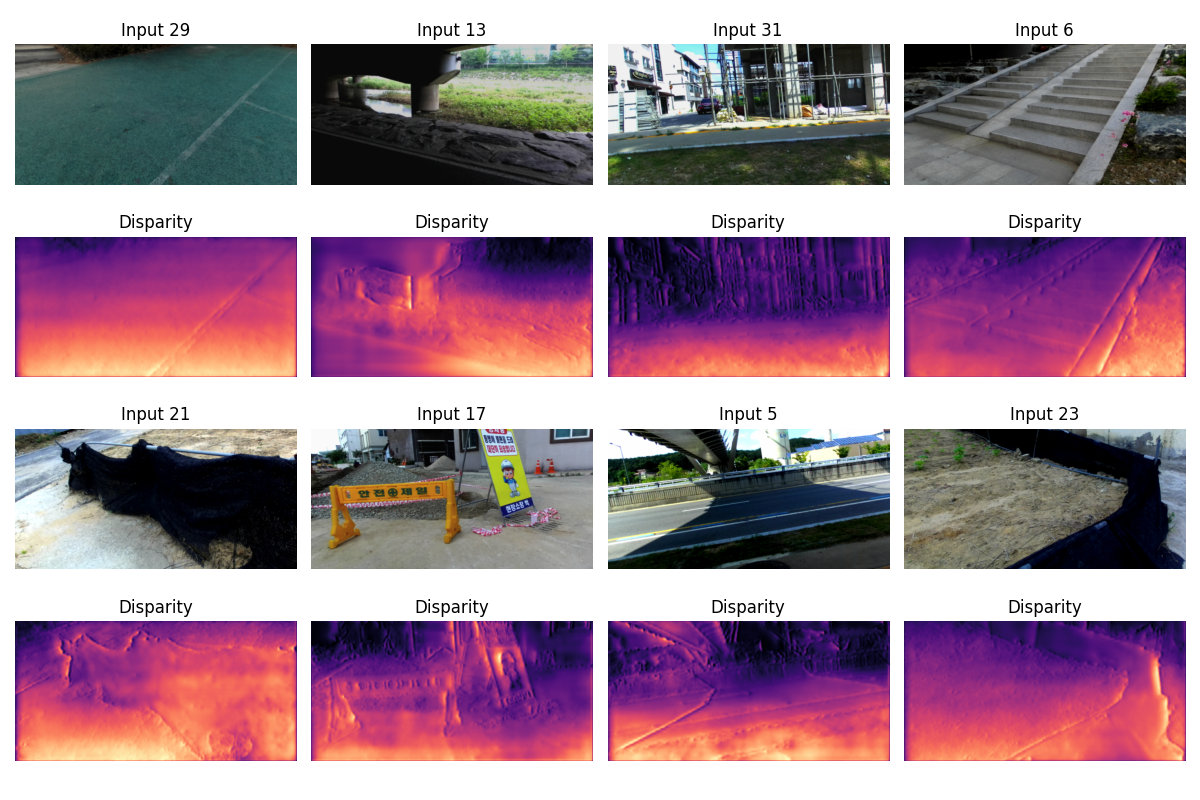
Figure 1: Depth predictions on eight random images from the DIML-RGBD dataset. Rows 1 and 3 are the input images. Rows 2 and 4 show disparity map predictions. These results were the best I could do with a budget of four hours of throwing everything I could at this problem.

Winter 2026, Rose-Hulman Institute of Technology

Instructor: Kyle Wilson

Overview

For the previous project we trained a neural network to predict depth from a single RGB image. Our dataset consisted of paired images with ground truth depth data. But these ground truth depth images are rather expensive to capture.

For this project we’re going to train a depth model the hard way: instead of ground truth depth data, we’ll work from images captured as stereo pairs.

This is self-supervised learning. We don’t have labeled ground truth, but we have a constraint: if our predicted depth is correct, then warping the right image using that depth should more or less reconstruct the left image. Your core challenge on this project will be to write a loss function that encodes that computation.

This is a group project. We’ll be using specialized hardware (GPUs) for training the models, and groups will help make sure there is enough compute to go around.

Learning Objectives

By doing this project, you will learn to:

• Understand the relationship between disparity and depth in stereo vision
• Implement a self-supervised photometric loss function
• Use differentiable image warping via grid_sample
• Apply techniques from the previous project to a harder problem

Technical Requirements

This project uses the same GPU server setup as the Depth1 project. Refer to the compute server documentation for instructions on:

• Installing VS Code and required extensions
• Connecting to Gebru via Remote SSH
• Setting up your Python environment with uv
• Server etiquette and GPU sharing

The starting code includes a pyproject.toml that will install the necessary dependencies. You’re welcome to continue using the same Python kernel that you created for the previous project.

Dataset

This project uses the DIML-RGBD outdoor stereo dataset. On the CSSE GPU servers, the data is pre-installed at /work/csse461/diml_rgbd_small/outdoor. If you’re working on your own machine, download the “sample data” from the DIML-RGBD website. The full DIML-RGBD dataset is much larger than the sample (so you could train a much better model!) but it’s hard to download, and all of your training runs would take ages. You’ll learn more by doing the best you can with this smaller dataset.

Core Tasks

I recommend completing these in order:

Task 1: Define a Model

Start by pasting in your best model from the Depth1 project. You may need to adjust some details for the different image sizes (256×512 instead of 240×320), or perhaps it will work as-is.

Important change: Your model now has a new task: instead of predicting depth directly, it will predict disparity (horizontal pixel shift). Notice that how little (perhaps nothing?) about your model needs to change.

A good idea: The starter code model uses F.softplus on the output to ensure positive values. This is a good choice for disparity prediction. If your depth model doesn’t end with softplus, consider adding it now.

Task 2: Stereo Loss Function

This is the core challenge of the project. Unlike Depth1, we don’t have ground truth depth maps. Instead, we use photometric consistency: if our disparity prediction is correct, warping the right image should reconstruct the left image.

There’s a hint if you’d like more guidance.

The Stereo Geometry

(The following section is a summary of material we’ll cover in class.)

A stereo pair is two cameras, pointed at the same scene, capturing images at the same time. In a rectified stereo pair, the two cameras point in the same direction (and that direction is perpendicular to the baseline between them). Our dataset was captured with a stereo rig: imagine two camera, bolted to a metal bar and facing the same direction, and rigged to both capture images simultaneously.

In a rectified stereo pair: - The left and right cameras are separated by a horizontal baseline - Corresponding points lie on the same horizontal scanline - A point at pixel (x, y) in the left image appears at (x - d, y) in the right image, where d is the disparity - Larger disparity = closer object (inverse relationship with depth)

What Your Loss Function Must Do

1. Create a sampling grid: Use the predicted disparity to compute where each pixel in the left image should sample from in the right image

2. Warp the right image: Use PyTorch’s grid_sample to resample the right image according to your grid. This creates a “reconstructed” left image.

3. Compute photometric loss: Measure how different the actual left image is from the reconstructed left image. L1 loss (mean absolute difference) works well.

Helpful PyTorch Functions

You’ll need to read the docs to figure this out. Each of these should be helpful:

• torch.meshgrid: Creates coordinate grids
• F.grid_sample: Differentiable image resampling (read the docs carefully!)
• torch.stack: Combines tensors along a new dimension

Don’t try to re-create any of the functions above! These functions are carefully coded to (1) be differentiable by pytorch, and (2) to run efficiently on a GPU. You don’t know how to do either of those.

Common Issues

• grid_sample expects coordinates in [-1, 1] range, not pixel coordinates. The starter code provides a normalized meshgrid to help with this.
• Watch the coordinate ordering: grid_sample expects the grid to have shape (N, H, W, 2) where the last dimension is (x, y) coordinates. Read the docs, and find examples to see how this works.
• Disparity scaling: Your disparity values need to be scaled appropriately to work with the normalized coordinate system. (i.e. a disparity of 8 pixels is a shift of \((2 * 8 / 256)\) if the image width is 256 pixels, and in a normalized coordinate system where -1 is the left edge of the image and 1 is the right edge).

Task 3: Train Your Model

Once your model and loss function are working, train your network using the provided training loop.

Here’s how you know if it’s working:

• No error messages or warnings

• The loss values should be decreasing over time

• Train and validation loss should roughly track each other

• The inference visualization should show disparity maps that make geometric sense – nearby objects should have higher (brighter) disparity

  Submission and Grading

Check-in

Upload sample output from your network to Gradescope. I’m looking for a visualization similar to the one at the top of this document. To meet this milestone, your code must be able to load data, compute the loss function without crashing, and produce disparity output that shows some structure (not just noise or constant values).

Code Submission

1. Commit: Turn in your code by committing to your GitHub repo, then posting your repo to Gradescope.
2. Artifact: Commit sample output (the .png files saved by the inference cell). I want to see your results without retraining your network.
3. README: Tell me which extensions you did (if any) in a short text file in your GitHub repo.
4. Weights: (optional) If you’re comfortable with it, commit a copy of your model weights so I can run your model too.

Grading Rubric

Minimum passing criteria: The loss function must be substantially correct. A submission with a broken loss function cannot pass, regardless of other components.

Possible Extensions

You’ll need to complete several extensions to get a high grade on this project. Extensions are graded for process, not performance. Show me the work you’ve done, even if the work didn’t lead to gains in performance. If you did the work and documented it then I can give you credit for it.

For a group of two, A-level work should be roughly three extensions of average size. You could also hit the same level of effort with two large extensions, or four rather small ones. Please talk to me if you’re unsure whether you’ve done enough!

Here are ideas for extensions:

1. Improvements to the Loss Function: Photometric (image appearance-based) stereo losses often result in noise depth predictions with “crinkly” artifacts. You can improve your loss function to reduce these and get better predictions.

   • Pre-blurring: Before computing the difference between the left image and the warped right image, blur both with a small Gaussian blur to reduce noise. (Faster variant: use a small average filter, like 3x3.)

   • Smoothness loss: Add a piece to your loss function that computes x and y derivatives of the disparity prediction. Sum up the magnitude of those derivatives, and incorporate that into your overall loss.

   • Edge-aware smoothness: Like the previous option, but instead of uniformly penalizing disparity gradients, allow sharp disparity changes where the image has edges (depth discontinuities often align with image edges).

2. SSIM loss: Replace or augment L1 loss with Structural Similarity Index (SSIM), which better captures perceptual image similarity.

3. Left-right consistency: Train with both left→right and right→left reconstruction, and enforce that the two disparity predictions are consistent.

4. Pre-trained encoder: Use a reference CNN, pre-trained on a very large dataset, as the encoder side of your model. Write your own decoder (upscaling layers).

5. More data: I’ve downloaded parts of the full DIML-RGBD dataset. The files are at /work/csse461/diml-rgbd. The full dataset is stored in a different file structure, so you’ll have to do some work to get them into your training loop.

6. Multi-task training: (I’m not sure this will work very well, but you’re welcome to try it!) Can you train a model on two tasks at once? Train it to do depth-from-single-image with fully supervised indoor depth data. Then also train it to make depth predictions given stereo pair supervision on outdoor scenes. The usual way to do this is to interleave the training: take a few gradient steps on problem 1, then take a few steps on problem 2. etc.

I haven’t exhaustively tried all extension ideas. I will say that the results at the top of this page came from a combination of improved loss (pre-blurring, edge-aware smoothness term) and a UNet-like model whose encoder side was a pre-trained ResNet18. I also found a few tricks from the previous project (weight decay, a Dropout layer in the bottleneck) useful.