| Table of Contents |
Crummett and Western, Physics: Models and Applications,
Sec. 45-4
Halliday, Resnick, and Walker, Fundamentals of Physics (5th
ed.), Sec. 43-3
Tipler, Physics for Scientists and Engineers (3rd edition),
Sec. 40-3
Your goal in this experiment is to determine the half lives of two radioactive isotopes of silver that are formed when ordinary silver is irradiated with slow neutrons.
The decay of individual radioactive nuclei is a random process. It follows that, if N0 is the number of unstable nuclei of one type present in a sample at time t=0, the number N still present at the end of time t is,
![]() (1)
(1)
where ![]() is a constant,
characteristic decay rate of the particular isotope. The "half life"
T½ of the nuclide is defined as the time for half of
the unstable nuclei to decay. Therefore,
is a constant,
characteristic decay rate of the particular isotope. The "half life"
T½ of the nuclide is defined as the time for half of
the unstable nuclei to decay. Therefore,
![]() or
or ![]() (2)
(2)
Thus ![]() (3)
(3)
Although it is usually not convenient to measure the number of undecayed nuclei remaining at time t, the rate of decay R = -dN/dt at any instant of time may be measured by determining the rate at which particles are being emitted by the nuclei. This decay rate is proportional at any instant to the number of undecayed nuclei in the sample at that instant, so
![]() (4)
(4)
where R0 is the decay rate at time t=0. Taking the natural logarithms on both sides of this equation gives,
![]() (5)
(5)
Thus if you plot the natural log of the decay rate as a function of time, the half-life of the isotope can be determined from slope of the resulting line.
In this experiment you will be looking at a sample of silver that is made radioactive by exposing it to slow neutrons. A complication is that silver contains two different radioactive isotopes, which decay at different rates. All atoms of a given element have the same number of protons in the nucleus (atomic number Z), but different isotopes of the element have different numbers of neutrons N in the nucleus. Isotopes are distinguished by adding the mass number to the chemical symbol, as a left-superscript (e.g., 20Ne and 22Ne) are isotopes of neon. Some isotopes of a given element are very stable and are found in nature; others are unstable and exist only for a short time after formation, changing into other isotopes by ejecting a particle (e.g. electron, alpha particle, etc.) from the nucleus.
In this experiment, a silver sample will be made radioactive by exposing it to thermal neutrons for a period of time. The experiment is to determine the half-lives of the radioactive isotopes by counting their beta decays with a Geiger tube.
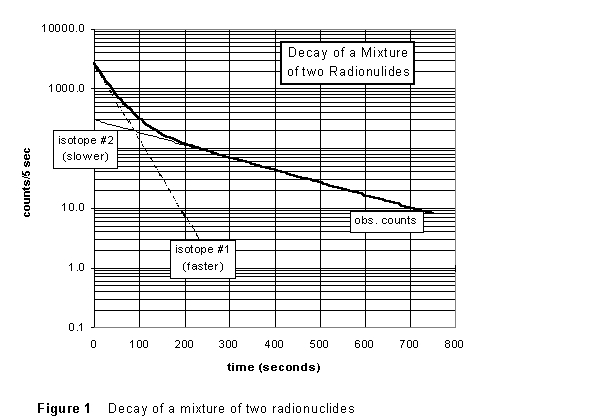
There are two radioactive isotopes formed when silver is irradiated, 108Ag and 110Ag; the two have different half-lives. This makes determining either half-life a bit more complicated. The decay might look like what is seen in Figure 1 below. In the later part of the data (after about t = 200 s), the logarithmic graph of the count rate vs. time appears to be a straight line, as Eq.(5) predicts. What's happened is that, by this time, the shorter-lived isotope has all decayed away, and we are just seeing the decay of a the longer-lived species. We could therefore use this part of the data to find the half life of the longer-lived nuclide.

Notice that the "opposite" is NOT true. During the first 250 sec both species are present, decaying at different rates, and we cannot extract the half life for the shorter-lived nuclide from this graph. The way we will deal with this is to use the late data to extract the value of the longer half life; then extrapolate this back to t = 0 and subtract off the counts in the early data that are due to the slower-decaying nuclide. What's left will be the decay curve for the short-lived nuclide alone. Finally, if we re-plot these data on a logarithmic graph, the slope will give us the half-life for the short-lived species.
Each station should have its Scaler-Timer turned on and connected to a Geiger tube, and the interface to the PC. Please do not make any adjustments to this apparatus. Call the instructor or the lab assistant if it does not appear to be behaving correctly. In particular, do not adjust either the voltage or the position of the Geiger tube.
| NOTE to instructors: A Geiger tube voltage of 800 Volts works well. |
(1) Before you count your irradiated silver sample, you must determine the background count rate at your station. Counting is done via a program geiger.exe in the c:\lab directory, or on a disk in the A drive. Type 'Geiger', and set up for counting by selecting item 5 on the main menu ('Set Geiger Parameters'). Then set a total sampling time of 60 seconds, with a count time/sample of 5 seconds. Make sure the counting station and Geiger tube are exactly as they should be (check with your lab instructor if in doubt) then return to the main menu and take data (for 60 seconds). When background counting is complete, go to menu item 2, 'Graph Count Rate vs. t'. Then by pressing the Ins key you will get the average of all the count rates displayed in the upper righthand part of the screen (the Ins key gives the average of the y-values between the cursors). This value should be recorded and then inserted in the program parameters (item 7 under 'Set Geiger Parameters'). From this point on, the program will automatically subtract the background count rate from the measured count rate.
(2) When you are ready to go, ask your instructor for a freshly irradiated silver sample. Do NOT handle the freshly irradiated samples yourself! Set the total counting time to something between 10 and 15 minutes (600-900 seconds), and the count time/sample at 5 or 10 seconds. Then have the instructor get a sample from the howitzer and place it in your counting chamber. Start your count as quickly as possible.
 (3) When
the computer is through counting, save your data set to a file. (Do this
immediately, before you forget! Most of the analysis you want to do on
the data will require spreadsheet software, or something equivalent, and
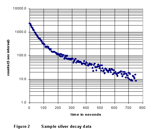
so you will want to do it off-line.) Display a semilogarithmic graph of
count rate vs. time; in its essential features, it should look just like
the example in Figure 2. Notice that the graph shows counts for 5-second
intervals. In the later data there are only a few counts in each interval,
with the result that the statistical fluctuations of the data are relatively
large. If you wish, in your analysis you can group several of the later-data
counts together into 20- or 30-second intervals.
(4) While still in lab, use the geiger.exe software to do a straight-line fit to the later data; remember you are looking for the asymptotic straight line. (If the data show a tendency to "curl away" (ether up or down) from a straight line at the very latest times, it probably indicates that an incorrect back-ground count rate was subtracted.) Record the equation of the line, and deduce from it a value for the half-life of the longer-lived nuclide (108Ag). Repeat, letting the other lab partner do the fitting. Clearly, from Figures 1 and 2, your result should be on the order of a few minutes.
(1) Import your data saved from GEIGER.EXE into a spreadsheet. If you feel it will make your data cleaner or clearer, group the later (t > 250 s) data in 20- or 30-second intervals. Make a graph of your data like that of Figure 2, showing count rate (logarithmically) as a function of time. Print out this graph (with appropriate size, labels, and features) and fix it permanently (use tape or glue, not staples!) in your lab notebook.
(2) Determine a least-squares straight-line fit to your later data, and from the parameters of the fit determine the half life of the longer-lived isotope (#2 in Figure 1) of radiosilver, WITH ERROR. How does it compare to the "eyeball" fits you did in-lab?
(3) Extrapolate the decay data for the longer-lived nuclide, using your best-fit line, all the way back to t = 0. From the equation for this fit to determine the number of counts due to isotope #2 in each of the intervals of your earlier data. Subtract this from your data in each interval; the difference is (presumably) the count rate due to the shorter-lived isotope (#1) only. Make a new logarithmic graph of these data for the isotope #1 alone, print out the graph and show it in your notebook. Do a second least-squares fit to THIS data, and from it determine the half life of the shorter-lived isotope, with error.
(4) From the two best straight line fits you have made, corresponding
to the decay curves for the two silver isotopes individually, determine
the initial (t = 0) count rate for each one. Since count
rate ![]() ,
,
![]()
you can determine the initial proportions in which radioactive atoms of each kind were formed by neutron bombardment.
Last rev 3/95