| Table of Contents |
Crummett and Western, Physics: Models and Applications, Sections 3-1, 3-2, 3-5
Halliday, Resnick, and Walker, Fundamentals of Physics (5th ed.), Sections 2-2 to 2-5
Tipler, Physics for Scientists and Engineers (3rd ed.),
Chapter 2
Introduction
This orientation is designed just to familiarize you with the apparatus that you'll use throughout this laboratory -- the Zenith PC's, the Sonic Ranger device and associated software, and their use to make measurements on objects in motion. The equipment is simple, in principle. The Sonic Ranger is a poor man's sonar, emitting ultrasonic "pings" and timing their echoes; the computer is a "smart" stopwatch-cum-scratchpad used to measure the time between reflected pings, write down data, transform and analyze it, plot graphs, etc., etc.
As you go through this exercise, keep notes in your laboratory notebook of what you do and what you observe, record all your results, etc. Your instructor may want to collect your notebooks and look over your work, but probably will not grade it.
When you turn on the Zenith 286 computer, it should (1) ask you to log onto the network and then (2) offer you a short menu of laboratory software available. When you log in with your personal user-name and password, the virtual "F: drive" maps to your personal space on the network. When the laboratory software menu comes up, type "get 1" to bring up the Sonic Ranger program RANGER.EXE (it is in the subdirectory LAB, so its complete DOS pathname is C:\LAB\RANGER.EXE.) The local hard drive on the Z-286 that you are working on is the C: drive, and the 3.5" floppy drive is drive A:). We will try to have the monitor color, focus, etc. adjusted on all machines; please let the instructor or an assistant know if anything needs tweaking.
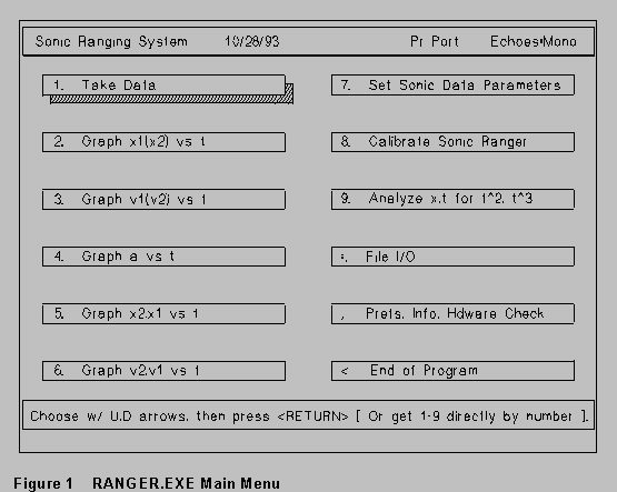
The main menu screen that comes up first is reproduced on the next page. This screen has a header line showing the name of the program, and two other pieces of information. (1) Either "PrPort" or "IO Box" will be showing, and (2) it will say "Echoes: Mono" or "Echoes:Dual". The sonic ranger can be driven either from the printer port, or the I/O Box; we will mainly be using the I/O Box, but you should check to see if your ranger is connected directly to the printer port at the back of the computer. (A ranger connected like this will have a cable to the printer port, and a thin cord to a small black transformer which plugs in an ac power outlet.) The "Echoes" message refers to setting the ranger to detect a single echo, or to detect two echoes. You'll see how to choose these options in a moment.
Item 1 on the main menu causes the machine to accept data from the sonic ranger; items 2-6 and 9 offer various choices for graphing and analyzing data; items 7-8 and 11 are used to set up the hardware and software; and item 10 is file input/output. Item 12 exits from the Sonic Ranger program to the DOS prompt.
.

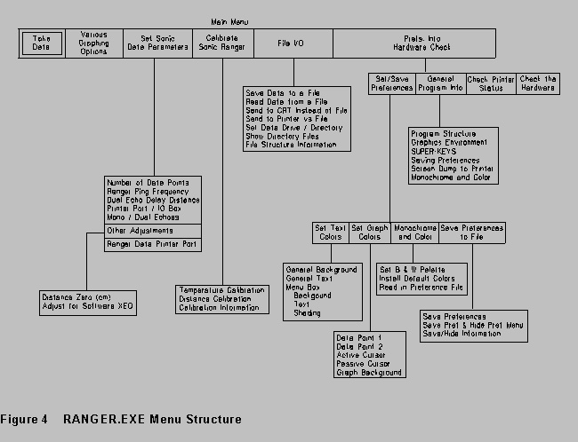
From this menu, select item 11 Prefs, Info, Hdware Check, and then select
General Info. Quickly read through items 1,2, and 4 from the
General Information menu. Item 4 will be useful for times when you do not
get all the echoes you would like.

Now return to the main menu. Under 7. Set Sonic Data Parameters, the
submenu for Ranger Parameters shows 7 items (including Exit to the "front"
menu). Note that items 4. and 5. permit you to toggle between selections
for driving the ranger, and between one and two echoes. Select
400 data points.
A ping rate of 80 Hz (pings/second)
IO Box (unless your pinger is connected directly to the printer port!)
'Mono' for single echoes (The 'dual echo delay' applies only when two
different objects are to be followed.)
Hit ESCAPE until you are back at the main menu, then select item 1, Take Data. An empty position vs. time (x-t) graph will appear. As you take data, it will appear directly on this graph.
Several items on this graph are important. One horizontal dotted line suggests that any target should be at least 0.4 m from the ranger. Another horizontal line at the very top of the graph gives the maximum range. The maximum range is dictated by the time between echoes, so the maximum range will increase as the ping frequency decreases. Near the top is a region in which echoes may be difficult to detect. The time scale at the bottom shows how long data collection will take at the given ping rate and number of data points selected.
Put your hand about half a meter in front of the Sonic Ranger, as a target. Press any key and the Sonic Ranger should begin to 'ping' (you may be able to hear very faint clicks, or buzzing, depending on ping rate). You should see data points registering on the screen as data is taken.
Note that the message at the bottom says "Retake data (y/n?)" when all data is taken. If you are satisfied with the data, press N and you will return to the main menu. From there you can look at graphs, and within a graph do editing, curve fitting, etc. If you wish to retake data immediately, just hit any key and the empty graph will appear, with the message at the bottom, "Press any key..." ([to begin taking data).
Try several other objects as targets, as well as your hand. Move the
targets toward and away from the Sonic Ranger. Try a flat target like a
book, and a skinnier one, like the edge of a book. Record all your observations
on this in your lab notebook. Are echoes equally smooth for all kinds
of targets, or does data "jump around" more for some targets
than for others? What is the best target for work in the two-to-four foot
range? Lower the ping rate and try some targets in the six-to-ten foot
range (the floor tiles are a handy way of estimating horizontal distance,
once you know their dimensions).
Editing and Graphing
Take a set of data on a moving target, and then return to the main menu by hitting N. Then select item 2, for the (x-t) graph. You are now in the "graph" environment, from which one may edit data, compare two graphs (one will be in the top half of the screen and the other will be in the bottom half; the graph choices are (x-t), (v-t), and (a-t)); or fit data with a straight line or a parabola.
(A data set contains just t and x values. The software computes v and a by simple difference formulas
 and
and  (1)
(1)
for the various displays.)
For a list of editing commands, hit F1. First, strike "E" for edit, and discover how the cursors work. These are vertical lines which delimit the part of the data set for analysis. PgUp selects the left or right cursor, PgDn changes the increment in the cursor when the right or left arrow is pressed (1, 10, 100 pixels), End plots just the section of the data between cursors, Home restores the full set of original data.
Find a section of the data which is looks pretty straight, and move the cursors until this data is between the cursors. Then give the command to replot this data. After the data is replotted, you may wish to fit it with a straight line. Call for the "line" fit, and a line will appear on the screen. The line has two cursors associated with it (one at each end) in the shape of circles. Try moving these cursors around, using commands which are very similar to the ones for the Edit cursors. Whenever you wish, you may call for the equation of the line. You may also toggle the line off with a command, if you get tired of seeing it on the screen.
Now return to Edit, and give the command to restore the full set of data. Find a spot on this data which has some curvature, and call for the Parabola fit. The parabola uses three cursors, which work much like the Edit and Line cursors. It is not as quick to draw the parabola on the screen, so a parabola will not appear until you call for it. As you adjust the cursors, no new parabolas are drawn until you specifically call for them. You can get the equation of the parabola whenever you wish, but remember that it goes through the positions of the cursors, and NOT through the previously-drawn parabola. If you ask for a freshly-drawn parabola, then ask for the equation, what you see is what you get.
The purpose of these curve fitting routines is to let you get an
immediate idea about your data while you are still in lab, and before you
have invested any heavy time in analysis. You will want to write down
the on-screen results in your lab book when you are about to save that
data to a file and do more work on it.
Saving and Transferring Data
You may save data files to various locations by choosing File I/O from the main menu. First select the data drive. If you are logged onto the network, and choose F:. (This may cause an error message, as RANGER.EXE doesn't know from the F: drive. Ignore it.) You will be saving to your personal mapped space on the network. Choose C:\DAT to save to the DAT subdirectory on the hard drive of the local Z-286 computer you are working on; select A: to save to the 3.5" floppy drive (careful about format; these are DD not HD drives)..
When you save your data to a file, You will be asked to give it a name. You will be invited to put in up to 80 characters of comments about this data, as a means of identifying it. After this, the routine saves the data you were last using to that file in the directory you have specified. Note it is possible to edit part of the data and save this to one file, and go back and re-edit to a different subset of the data and save that to a different file.
As an exercise, create a small (50 data points) data file, and send
it to your F: drive on the server.
Studying position, velocity, and acceleration.
(a) As a warm-up, predict what the graphs of x vs. t and
v vs. t will look like for a stationary object, and
make small sketches in your notebook. When that is done, take some data
for a stationary object (like a wall or a chair), and check that the graphs
in the computer are similar to the ones that you drew.
You have probably noticed that there is often some 'jitter' in the (x-t)
data, and that this produces glitches in the (v-t) graph which are
sometimes fairly wicked. Some of the jitter is due to software timing,
waiting to see if the ECHO line of the pinger has gone high, and some of
the jitter is due to irregular returning echoes from the target. Another
complication which will also show up is that your pinger may pick up sounds
from other pingers - and this WILL mess up your data.
The velocity and acceleration points are gotten from very simple difference
routines (Equations (1) above). We wind up with two fewer velocity values
than positions, and fewer less acceleration values than velocity values.)
When data is saved to a file, only the x vs. t data is saved. The
computer's (v-t) and (a-t) graphs are just to give you an
idea of what's going on, with minimal processing.
(b) The graph of velocity vs. time for constant-velocity motion is a
straight horizontal line. For this very simple motion, make a small sketch
in your notebook of what you expect for the graph of x vs. t. Now
move your hand or other target at what you think is constant velocity until
you get some reasonable-looking data. If this data fits what you and your
partner think the (x-t) graph should look like, then get back to
the main menu, and into the (x-t) graph (item 2 on the main menu).
Figure out a way to determine the velocity from this graph. You can use
simple multiplying and dividing as a check on what the Line function gives
you.
At this point, you could get back to the main menu and go from there
to the (v-t) curve; but instead, just go to Compare and get both
(x-t) and (v-t) graphs on the screen at the same time. The
velocity values should fall in the same general range you got before. (Do
they?)
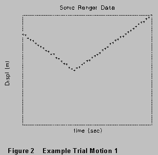
Now try making a graph that shows motion with constant velocity with
a reversal of direction -- the (x-t) graph would look something
like Figure 2 on the next page. Work on this until you get the constant-velocity
sections pretty straight and the reversal (the "corner") pretty
sharp. Try to get about the same velocity coming and going.
For this motion, what should a graph of v(t) look like? Make
a small sketch of the anticipated (v-t) graph in your lab
notebook before you begin. Take data until it looks about right in x
vs. t . Then see if the (v-t) graph also looks like what you
expected. What do you think the acceleration vs. time graph will
look like? Take a look at it! Record your observations and conclusions.
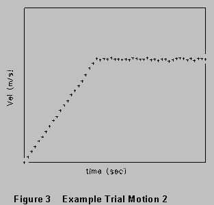
Shown in Fig. 3 is a different motion, this one on a graph of velocity
vs. time. Try to generate a sonic ranger graph of v vs. t which
looks like it. Before you start out, make a small sketch in your lab notebook
of what you think the (x-t) graph for this case should look like.
Take the minimum velocity to be zero.
(c) In this part you will try to make a target move with a small constant
(1 or 2 m/s2) acceleration. Before you generate any data, make
small of what you think the x vs. t, v vs. t, and a vs.
t graphs will look like. Then go ahead and try your hand at it.
When you get some (x-t) data which looks reasonable to you, try to determine the value of the acceleration. Try to get a value from the (x-t) graph (helped by curve fitting), from the (v-t) graph (with or without curve fitting) and -- if possible -- the (a-t) graph. Record your observations and conclusions.
Familiarization exercise - DOS software.wpd
last rev 7/97