| Table of Contents |
Welcome to spreadsheets! Very likely you have already used some spreadsheet software. If not, you'll find them very useful for tabulating, analyzing, graphing, and fitting experimental data. This brief introduction is written based on EXCEL 5 for Windows, which is widely available at the Institute. But other popular Windows-environment spreadsheet software such as Quattro Pro, differing in details, operate similarly.
You will find a lot of useful things you can do with spreadsheets in physics and physics labs; but if you've never used one before, you may think it's a lot of bother to learn how. It isn't.
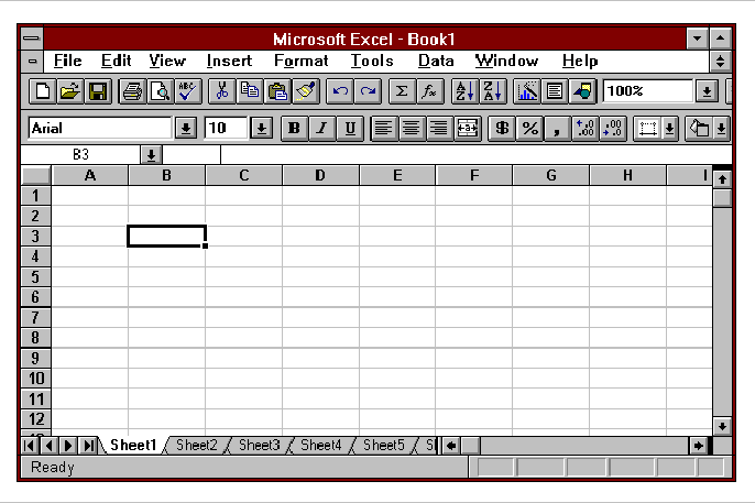
When you bring up EXCEL, you'll be faced with an empty spreadsheet, like that shown below, with the "Ready" prompt in the lower left corner. It is just an empty data table, like a blank bookkeeper's ledger, with row (1,2,3,4,...) and column (A,B,C,D,....) labels. Actually you're only looking at one corner of the spreadsheet; it can extend to hundreds of rows and columns.

To use the program, you'll first enter data into the cells of the spreadsheet, then execute various commands that appear on menus. Since this is a Windows application, there is always a Help button available if you forget how to do something.
Data are stored in cells. The spreadsheet display is a two-dimensional array of cells. Cells are organized by row and column; thus B3 is the third cell down in the second (B) column. The emphasis box (on cell B3 in the figure) identifies the active cell.
A cell is one of the storage locations in the spreadsheet; it may contain a quantity (4.62378), a date (30 May 1993), a label (VELOCITY), a formula such as (A13+2.2*@SQRT(B3)), etc.
To enter stuff, get to the READY screen if you aren't already there, go to the cell you want (just mouse-clicking on the cell is the easiest way), and just type in your stuff (number, text, or date), and hit ENTER. To EDIT what's already in the cell, double-click on that cell (or hit F2). Make whatever changes you want. If you want to delete all or part of what's there, select that part -- click the mouse button at the beginning, hold it down, and drag -- then press Del. When you're done, hit ENTER.
You move around from cell to cell using the arrow keypad. For vertical giant steps (a screen at a time), PgUp and PgDn; for horizontal giant steps, Alt + PgUp or PgDn. Ctrl-Home goes to the first cell (A1), Ctrl-End to the last non-empty cell. F5 is the GO STRAIGHT THERE key. As always in Windows applications, the scroll bars help you navigate also.
For operations like cut, copy, etc., you can select a block (a rectangular group) of cells. A block is designated by upper-left-corner and lower-right-corner cell addresses (e.g. A2..D31).
Basically, like all Windows applications, EXCEL is menu-driven; when the program is at READY, the main menu is spread out across the top of the screen. The entire capability of the program is organized by a system of menus that branch off from this one.
To choose one of the pull-down sub-menus, just click on it. For instance, clicking on Edit drops down the Edit menu, which contains commands to Cut, Copy, Paste, Delete, Go to, etc., etc., then clicking on the command you want to execute. You can also access menu selections by moving the cursor to the desired menu option, then pressing ENTER or RETURN.
Pressing ESC will always back you out of wherever you are, to the previous menu. ESCing repeatedly will take you all the way back to the READY condition.
To make this even easier, the most common menu functions are displayed on a "button bar" across the top of the screen, just below the main menu line. The functions of the buttons on the main bar are spelled out in the chart on the next page: for example, pushing the second button has the same effect as the menu choices File Open.
| NEW WORKSHEET -- Creates a new empty worksheet. | OPEN -- Loads an existing worksheet that has been saved as a file somewhere. | ||
| SAVE -- Saves the worksheet currently displayed to a file. | PRINT -- Prints the worksheet currently displayed to the selected printer. | ||
| PRINT PREVIEW -- Displays the current worksheet as it will appear when printed. | SPELLING -- Starts the spelling checker. This checks text and number cells against an internal dictionary. | ||
| CUT -- The currently selected range is cleared and transferred to the Clipboard. | COPY -- The currently selected range is copied to the Clipboard. | ||
| PASTE -- The contents of the Clipboard are entered into the worksheet, beginning at the currently active cell. | FORMAT PAINTER -- Copies formatting to a range of cells. | ||
| UNDO -- Undoes the last command. | REDO -- Repeats the last command given. | ||
| AUTO-SUM -- Sums the values of a range of cells. | FUNCTION -- Starts the "Function Wizard" -- that is, starts a function call. | ||
| SORT ASCENDING -- Sorts selection in ascending order. | SORT DESCENDING -- Sorts selection in descending order. | ||
| CHART -- Starts the "Chart Wizard" -- that is, begins the creation or editing of a graph (Excel calls them charts). | TEXT BOX -- Creates a text box. | ||
| DRAWING -- Displays the Drawing toolbox. |
| ZOOM -- Zooms the worksheet to the size you specify. |
Suppose we want to calculate x = ½ at2 + v0t, for values of t = 1,2,3,...,10. The first thing to do is put the t values in cells A6 ... A15. The straightforward way to do this is to use a formula to increment each cell. Here, for example, enter 1 on cell A6. Then enter the formula =A6+1 (the equal sign is Excel's flag for a formula); when you do so, a 2 appears in cell A7. Now copy the formula from cell A7 into cells A8 through A15. To do this, click on cell A7, then choose Edit Copy (or click on the Copy button on the tool bar). Next select (hold down the mouse button and drag) the range A8 ... A15. Finally, choose Edit Paste (or click the Paste button) to "paste" copies of the formula into the selected cells. Note that if you click on cell A8,A9,A10, ... the formulas there are NOT =A6+1, but
=A7+1
=A8+1
=A9+1
-- Excel has updated the cell reference each time it copies it. This is probably the coolest thing about spreadsheets!
A sexier way to do this is to fill the range. First enter the first two numbers: enter 1 in cell A6 and 2 in cell A7. Then select the two cells (A6 and A7) containing the first two entries. Point to the AutoFill handle (the little square at the lower right corner of the select box), drag the cursor down through A15, and release the mouse button. Excel will fill in the sequence of numbers.
The acceleration a, and the initial velocity v0, are constant. In SI units, the acceleration of a freely falling body has the value g = -9.81; enter this in cell B2. Let's suppose you throw the object up in the air at a speed of 44 m/s; enter 44 in cell B3. In cell A2, enter g = and in cell A3, enter v0 =. This is an example of labeling things on your spreadsheet.
In cell B6, you're going to put a formula to calculate x from the value of t in A6. Go to cell B6, and type
=0.5*$B$2*A6^2+$B$3*A6
Excel will evaluate the formula (take whatever's in cell A6, square it, multiply what it gets by whatever's in cell B2, multiply that by 0.5, take what's in A6, multiply it by what's in B3, add it to the first term) and display the numerical result (39.095) in cell B5 on the screen. This is the value of x corresponding to the time (t = 1) which is in cell A6. (Why did we decorate the cell addresses B2 and B3 with dollar signs? We'll see that in a minute.)
Now copy the formula in A6 into cells A7 ... A15. The next thing you need is a similar formula in cell B6, to calculate x for the time value in A6. You can copy A6 into the range A7 ... A15 just as you did above. Select cell A6, then choose Edit Copy (or click on the Copy button on the tool bar). Next select the range A7 ... A15. Finally, choose Edit Paste (or click the Paste button) to "paste" copies of the formula into the selected cells.
Again, if you look in cell B7, B8, B9, ... the formulas there are each updated: Excel has automatically changed the row numbers as it copied the formula each time, so that the formula in B7 calls for the time value from A7, the formula in B8 calls for the time value from A8, and so on. Notice that the addresses of the constants g and v0 didn't change; when you wrote the first formula you flagged that address with dollar signs, to tell Excel "this is an absolute address; don't adjust it."
Another snazzy thing about a spreadsheet is that what you enter, a lot of the time, is not a value but a relationship between values. For instance, just now, you didn't calculate x values and then enter them; you entered a formula, and let Excel calculate the x values from it. If you change something, the spreadsheet automatically reevaluates the formulas.
In this case, your formula involved a constant, g, the acceleration due to gravity. Suppose you wanted to tabulate the positions of a falling body on Mars, where g = 3.71 in standard units. All you have to do is enter -3.71 for g in cell B2, and the calculations are immediately redone for you. (Try it and see!)
At some point you'll want to make a graph of your results. Excel calls graphs "charts". To graph x vs. t for our example here, first mark the block of data you want to graph; here, cells A6 to B15. (Excel wants data series in a block of adjacent columns. Here the independent variable values are in A6-A15, and the dependent variable values in B6-B15.)
Now hit the Chart Wizard button on the main toolbar. ( "Wizard" in Excel is a little program that carries out the basic steps of a task for you.) Nothing much happens. Mark (click and drag) the unused block of the spreadsheet where you want the embedded graph to appear: let's say, D3-H16. When you release the mouse button, the ChartWizard dialog box appears. It will (1) ask for the range of data to be graphed; (2) ask you what type of chart you want (in plotting scientific data you almost always want the XY chart), then ask you for a few more particulars. When you finish its steps, your graph will appear.
You can edit, augment, modify, and prettify your graph to your heart's content. Double-click on any feature (the x-axis, say) and a dialogue box for that feature appears; open the Insert menu while the graph is active, and you can add other features to your graph.
While you're at it, take a few minutes to play with as many of these features as you can find, and see what you can make your graph do.
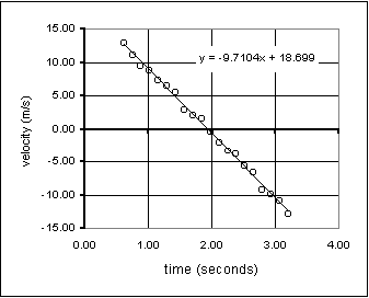
Often, individual data values that you measure aren't what you want from your experiment; rather it's the trend of the relation between the variables. The data graphed at the top of the next page show the velocity of an object in free fall vs. time. Velocity values aren't what we want to know here; we want the acceleration of gravity, which is the slope of a straight line through the data. Excel will easily generate the best straight line through the data, as shown in the graph; similar functions are available in other full-featured spreadsheet programs.
Notice that a "connect-the-dots" track is NOT what you want. That will not show anything useful, and will give your lab instructor heartburn.
When you've built your graph, add a "trend line" as follows:
 Click on "Insert
Trendline". A menu box will appear that lets you select the type of
fit you want to apply to the data (linear, logarithmic, quadratic, etc.)
And you have various options, such as whether or not to display the equation
of the fit on the graph (this has been done in he example at left).
 This procedure is very much easier than using the more powerful regression tools that are available in Excel. Its one drawback is that it provides no error estimates for the trendline coefficients. (A goodness-of-fit parameter R2 is, however, available on the Options menu.)
If you have a graph made, adding a trend line is the quickest way to get a best-fit straight line. If you don't need a graph but just want the parameters of the best-fit line, the functions SLOPE and INTERCEPT accomplish this easily.
In building your formulas, you can use the operators +, -, *, /, and ^ for exponentiation. There are also a number of mathematical functions you can use which Excel will recognize. For instance, SIN(B23) produces the sine of whatever quantity is in cell B23. (The quantity will be treated as if it were an angle in radians.)
Some of the more common mathematical and statistical functions that you can use in Excel formulas are
ABS(number) -- returns the absolute value of a number
ACOS(number) -- returns the inverse cosine of a number, as an angle in radians
ASIN(number) -- returns the inverse sine of a number, as an angle in radians
ATAN(number) -- returns the inverse tangent of a number, as an angle in radians (two quadrants)
ATAN2(x,y) -- returns the inverse tangent of (x,y) coordinates
AVERAGE(list) -- returns the average of the arguments
COS(number) -- returns the cosine of an angle expressed in radians
COUNT(list) -- counts how many numbers are in the list of arguments
COUNTIF(list) -- counts how many cells in list meet given criteria
DEVSQ(list) -- returns the sum of squares of deviations from the men
EXP(number) -- returns the exponential function of a number
FACT(number) -- returns the factorial of a number
IF(test,value,value) -- performs a logical test
INT(number) -- returns the integer portion of a number
INTERCEPT() -- returns the intercept of the regression line
LN(number) -- returns the natural logarithm of a number
LOG10(number) -- returns the base-10 or common logarithm of a number
MAX(list) -- returns the maximum value in a list of arguments
MIN(list) -- returns the minimum value in a list of arguments
MINVERSE() -- returns the inverse of the specified matrix
MMULT() -- returns the product of two specified matrices
NORMDIST() -- returns the normal distribution function value
PI -- returns the value of pi = 3.1415926....
RAND -- returns a random number between 0 and 1
SIN(number) -- returns the sine of an angle expressed in radians
SLOPE() -- returns the slope of the regression line
SQRT(number) -- returns the positive square root of the given non-negative number
STDEV(list) -- returns the sample standard deviation of the values
SUMSQ(list) -- returns the sum of the squares of the arguments
TAN(number) -- returns the tangent of an angle expressed in radians
VAR(list) -- returns the sample variance
There is a "Function Wizard" (fx on the main toolbar) which will present you with a list of all the functions available in Excel, allow you to select your function, and lead you through its use.