Michael J. Moloney
Department of Physics and Applied Optics
Rose-Hulman Institute of Technology
Terre Haute, Indiana 47803
moloney@rose-hulman.edu
(Copyright 2002, Michael J. Moloney)
Abstract. I. D. Johnston1 laid out a group of diverse, interesting acoustical calculations, done in a computer program using second order Runge-Kutta integration. All of these can be readily done on a spreadsheet, which may be a more advantageous platform, given its near-universal accessibility, its built-in graphing, and its means of immediate feedback when parameters are changed.
Introduction. Ref. 1 presented a rich array of (essentially one-dimensional) acoustic resonance calculations in the context of a straightforward computer program, including treatment of
Inserting a Scroll Bar. To insert a scroll bar in ExcelÔ , one goes to View/Toolbars/Control Toolbox (in older versions View/Toolbars/Forms) . This brings up a toolbar with a variety of 'controls', including scroll bars. One clicks on the scroll bar, goes to a free area on the spreadsheet and drags a rectangular area for the scroll bar. Now the scroll bar must be connected to a cell, and set to the proper range. One pops up a menu by right-clicking on the scroll bar, then selects Properties (Format Object in older versions). Now the user enters the Linked Cell and also the scroll bar Max and Min values . The integer values in the linked cell are then converted via formula into the desired parameter in some other cell .
It is convenient to have one scroll bar for Coarse Frequency and one for Fine Frequency. For a pipe open at the far end, one may also want the pressure in the last cell and the flow rate in the last cell to be shown at the top of the sheet near the frequency scroll bars. This will enable the user to fine-tune the desired value as close to zero as possible.
One-Dimensional Acoustics1. The variables of interest are pressure p and volume flow rate U = Sv, where S is the cross-sectional area, and v is the acoustic velocity. Following Ref. 1, we take each as a one-dimensional wave of the form g(x,t) = A exp(iw t-ikx). Two first-order linearized equations for acoustic behavior are needed. The first comes from Newton's second law:
-¶ p/¶ x = r ¶ v/¶ t .
For a discrete interval D x, we approximate D p by
D p = -Z U , (1)
where Z = i D x rw
/S is referred to as the pipe impedance. (r
is the fluid density.)
The second equation comes from the equation of continuity
-¶ U/¶ x = S/B ¶ p/¶ t,
where B = g Po is the bulk modulus, (Po is atmospheric pressure and g is the ratio of specific heats at constant pressure and constant volume). For a discrete interval we approximate D U by
D U = -Y p , (2)
where Y = i D x S w
/(g Po) is the pipe 'admittance'.
Equations (1) and (2) provide the rates of change for p and U. If p is assumed real, U, Z, and Y may be taken to represent the imaginary parts U, Z, and Y respectively1. This effectively changes the sign of (1) when implemented in the spreadsheet:
pk+1 = pk + Zk+1/2 Uk+1/2 and
Uk+1 = Uk - Yk+1/2 pk+1/2 .
If S is constant, Y and Z need be evaluated only once, not at each step or half-step. In this situation, the calculations can be folded together to give
pk+1 = pk (1 ½ YZ) + Z Uk ( S = constant) and
Uk+1 = Uk (1 ½ YZ) - Y pk ( S = constant) .
For constant S, the folded RK2 requires only a column for distance, one for p and one for U. When S varies, the RK2 equations are not readily folded, and several more columns are needed.
In the authors sample spreadsheet3, S is constant, and only three columns are used, plus one additional column to provide for any holes which may be present. At an open end1, an 'end correction' is applied to effectively increase the length.
Finger holes. At a hole in a pipe the additional flow through the hole is dealt with by adding an 'admittance' Yhole for the hole (in addition to Y for the pipe). The hole admittance is placed in a column kept empty except for the locations of holes. In Ref. 1, Yhole is given by
Yhole = rhole/(2.8 ro f),
where f = w /(2p ) is the frequency and ro is the equilibrium density of air . When the factor (1-YZ/2) is calculated for each step, Y is set equal to the admittance of the column plus Yhole.
To test the spreadsheet with holes present, three holes were drilled in a PVC pipe and resonant frequencies were measured for six different configurations of holes open and closed. Initially there was trouble fitting the frequency of even one open hole. To resolve this problem, it was necessary to change the sign of Yhole as given in Ref. 1. Then Yhole was modified for the presence of pipe thickness. For a hole of radius r and wall thickness t, the form used was
Yhole = -r2/(r+Dt)/(2.8 ro f),
where f is the frequency in Hz, and D is an adjustable constant, expected to be near 0.7. With this form, and adjusting for room temperature, the spreadsheet was able to match all six resonant frequencies within 1% using one adjustable parameter D.
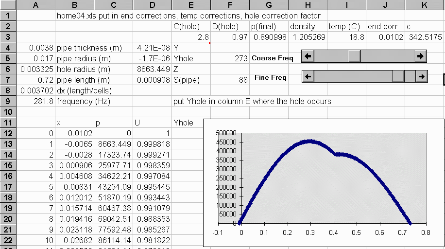
Fig. 1 shows part of a spreadsheet of 201 cells for a pipe of physical length 0.72 m, open at both ends, with a hole 0.41 m from one end. (This sheet is not the sample spreadsheet of Ref. 3. It has had a temperature correction added.) Notice that the pressure starts at a negative value of distance, due to the way the end correction was added. Pressure values are unrealistically high due to the nominal starting flow rate of 1 m3/s.
Sample Acoustic Resonance Spreadsheet. A sample spreadsheet pipetest.xls is available at http://www.rose-hulman.edu/~moloney. This was written in Excel 5.0 and so should run on more recent Excel versions. One simple item not included in Ref. 1 or in this sample spreadsheet is a temperature correction. This would make a nice exercise for students, so that results are adjusted to ambient temperature.
References.
1. I. D. Johnston, "Standing Waves in Air Columns: Will Computers Reshape
Physics Courses?" Am. J. Phys, 61. 996-1004 (1993)
2. C. W. Misner and P. J. Cooney, Spreadsheet Physics, (Addison-Wesley,
Reading Mass, 1991)
3. Pipetest.xls ( a sample spreadsheet) available at http://www.rose-hulman.edu/~moloney

Figure 1. Part of a spreadsheet for resonance in an open-open pipe with
one hole.