Divorce and Female Labor
Force Participation:
Evidence from Times-Series
Data, Causality Tests, and Cointegration
I. Introduction
Divorce, female labor force
participation, and median real annual income for females are important
indicators of the economic status of women in the
The sizable increase in the number
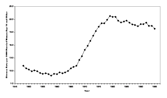
of divorces (see Figure 1) has led to much research and conjecture regarding
the factors that influence the decision to dissolve a marriage. This increase has been attributed to, among
other factors, the sexual revolution of the Sixties, the emergence of no-fault
divorce procedures, the diminished stigma associated with being divorced, and
the increased acceptance of divorced individuals as suitable spouses. However, early researchers placed a great
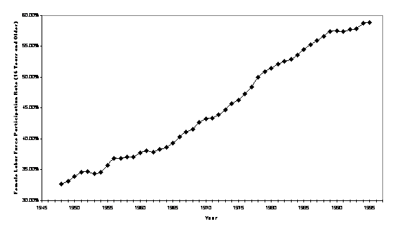
deal of emphasis on the idea that increasing female labor force participation
(see Figure 2) placed various “pressures” on the household and, ultimately,
resulted in larger numbers of divorces.
Closely tied to this argument is the indisputable relationship between
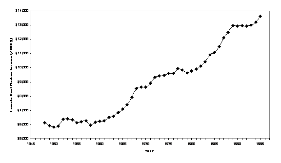
income and labor force participation. As
female incomes rise (see Figure 3), divorce, the argument goes, becomes more
likely.
Using time-series techniques, this paper
investigates the relationship between divorce, female labor force participation,
and median female income. Though it is
shown that these variables exhibit unit roots, their first differences are
found to be stationary, and evidence is produced that they are cointegrated. In other words, the cointegration techniques
of Johansen and Juselius show the existence of a long-run relationship between
these variables.
A VAR of the first differenced data is
estimated using an error-correction technique.
Impulse functions from this model reveal that an increase in divorce
leads to a rise in female labor force participation; but, positive innovations
to female labor force participation imply a decline in the divorce rate. Impulse function analysis also shows that a
positive innovation to median female income leads to increased divorce and
increased labor force participation on the part of females.
The rest of the paper consists of five additional sections. Section II provides a relatively thorough review of the literature regarding marital dissolution. Section III gives a complete discussion of the data and its sources along with the unit roots tests for the various time series. The fourth and fifth sections present the cointegration and the vector error correction model results. Finally, in Section VI, conclusions and recommendations for further research are provided.
II. Literature review
There have been many studies of divorce in
the
Lombardo [1999], and Greene and Quester
[1982] argue that wives facing a higher risk of divorce will hedge against that
risk with higher levels of labor force participation, and that they will also
respond by working longer hours. The
basic argument made in these papers is that investment in nonmarket activities,
such as child rearing, becomes relatively less attractive (it yields a lower
expected return), and investment in human capital becomes relatively more
attractive (it yields a higher expected return) as the probability of divorce increases. Studies by Johnson and Skinner [1986], and
Shapiro and Shaw [1983] provide additional evidence for the above argument by
finding that women increase their labor force participation prior to
dissolution of a marriage. The above
papers make a clear causality argument that an increase in the likelihood of
divorce increases a females willingness to enter the labor force.
Spitze and South in two separate studies
[1985, 1986] argue a different line of causality. Their conclusion is that an increase in
female labor force participation leads to an increase in familial conflict and,
consequently, an increase in divorce.
Substantiating evidence for this view is provided by Mincer [1985] who,
in a survey of twelve industrialized nations, found that rising divorce rates
clearly lag rising female labor force participation rates.
Previous studies of the impact of income
on divorce have provided mixed results.
Becker, Landes, and Michael [1977] find that a rise in expected female
earnings increases the probability of divorce, while a rise in expected male
earnings reduces the probability of divorce. D’amico [1983] recognizes two
distinctly different possible effects of income on divorce. One hypothesis is that as the female’s wage
relative to the male’s rises, conflict based on competition for status within
the marriage will occur and will increase the likelihood of divorce. The second, opposing hypothesis, is the
notion that the pursuit of higher socioeconomic status is a familial one and
that a wife earning a relatively higher wage than that of the husband may
contribute to the overall status goal and solidify the marriage. D’amico’s results tend to confirm the latter
hypothesis. Finally, Hoffman and Duncan
[1995] find no support for the hypothesis that increased real wages for females
lead to increased divorce rates.
However, Spitze and South raise another
question that is closely related to the income issue. In a 1985 study, they produce evidence that
the number of hours a wife works has a greater impact on the probability of
divorce than do various measures of the wife’s income.
Using time-series analysis, South [1985]
finds little evidence that the divorce rate rises during periods of recession
and falls during periods of expansion.
He does find a positive, albeit small, effect of unemployment on the
divorce rate. His model indicates that
changes in the age structure and the labor force participation rate of women
have significantly stronger impacts on the divorce rate than other
macroeconomic variables.
Finally, using a simple vector autoregressive (VAR) approach, Bremmer and Kesselring [1999] show that the female labor force participation rate does not Granger cause divorce rates. However, they do provide statistical evidence that divorce rates Granger cause female participation in the labor force. They also show that past participation in the labor market influences women salaries.
III. The data and unit root tests
Annual time-series data for the divorce
rate, the female labor force participation rate, and the level of median real
female income are readily available.
Data on the divorce rate was obtained from the National Center of Health
Statistics of the Centers for Disease Control.[1] The level of real median female income was
acquired from the U.S. Census Bureau.[2] The labor force participation rate for women
sixteen years and older was obtained from the Bureau of Labor Statistics.[3]
One of the main contributions to the study of macroeconomic time-series is the importance of verifying whether a time-series is stationary. Time series that are nonstationary have unit roots and can be characterized as random walks. In regard to regression analysis, if both the dependent variables and the independent variables are nonstationary, spurious results may occur. In this case, traditional statistical inference using standard t-tests and F-tests would tend to reject the hypothesis that there is no relationship between the dependent and explanatory variables when, in fact, no underlying relationship between the variables exist.[4] To ensure that inferences from time-series regressions are valid, one has to statistically test whether the data series exhibit unit roots. To accomplish this, the augmented Dickey-Fuller [1979] test and the Phillips-Perron [1988] test are used.
Let Z be a time series variable. If Z
follows an autoregressive scheme, then Zt = ρZt-1 +
ut, where ![]() , and ut is a white noise, random error term. If Z follows a random walk, then Z has a unit
walk, implying ρ = 1. The augmented
Dickey Fuller test detects unit roots by estimating the regression
, and ut is a white noise, random error term. If Z follows a random walk, then Z has a unit
walk, implying ρ = 1. The augmented
Dickey Fuller test detects unit roots by estimating the regression
![]() (1)
(1)
where t is a time trend, ΔZt = Zt – Zt-1, and εt is the error term. In equation (1), δ, β0, β1, and ωi, i = 1, ... , m, are regression parameters to be estimated. The null hypothesis of a nonstationary random walk implies δ equals 0. The number of lagged dependent variables included as explanatory variables depends on how long the lag length needs to be to ensure that εt is not serially correlated.
The results of the augmented Dickey-Fuller tests are reported in Table 1. In the case of all three of the variables - - the divorce rate, the female labor force participation rate, and the median female real income - - the null hypothesis of a zero root is not rejected. However, the first differences of this data do appear to be stationary. In the case of the first differences of the divorce rates, the null hypothesis of a unit root is rejected at the 10 percent level. The null hypotheses of unit roots in the first differences of the female labor force participation rate and median real female income is rejected at the 1 percent level. Given the statistical evidence that the first differences of these data series are stationary, these variables are said to be integrated of order one, or I(1).
Further evidence that the first differences of these variables are stationary is shown in Table 2, which shows the Phillips-Perron unit root tests. This test differs from the augmented Dickey-Fuller test by correcting for autocorrelation parametrically, thus preserving the larger sample sizes by not having to add lagged dependent variables to eliminate autocorrelated error terms. Using levels data, this tests fails to reject the null hypothesis of unit roots for all three of the variables. However, once the data is first differenced, the Phillips-Perron tests indicate that all three series are stationary. Using first-differenced data, the null hypothesis of unit roots is rejected at the one percent level for first-differences in the female labor force participation and real median female income. The null hypothesis of nonstationary is rejected at the five percent level in the case of first differences of the divorce rate. Therefore, in a finding that is consistent
with the augmented Dickey-Fuller results, the Phillips-Perron test results reported in Table 2 indicate that each of these three data series is I(1).
IV. Cointegration tests
If the three time series--divorce rate, female labor force participation rate, and median real income--all have unit roots, a vector autoregression (VAR) of these variables may lead to misleading, spurious results. However, there may exist a linear combination of these variables that is stationary. This stationary, linear relationship of the nonstationary time-series variables is called a cointegrating equation, and it is often interpreted as the true, long-run relationship between the variables.
The increasing prevalence of VAR’s in time series estimations derives from the problems usually confronted by economists wishing to avoid specification errors common to most time-series methods. For most econometric models, the choice of specification can be a very thorny issue. The typical specification search is strictly one of trial and error. Frequently, different functional forms and combinations of possible explanatory variables are selected and tested. The reason for this is that economic theory may not conclusively indicate the impact of a given variable, nor may it conclusively indicate which variables should be included in--or, for that matter, excluded from--the model’s specification. Furthermore, theory may do little to reveal the true functional form of the model.
Therefore, to minimize the possibility of specification errors, to exploit the simultaneity of the variables chosen for the model, and to circumvent the possibility of making incorrect distinctions between exogenous and endogenous variables, a VAR model was chosen to explain the relationship between the divorce rate, the female labor force participation rate, and the level of median real female income. In a VAR framework, each endogenous variable is a function of past values of all endogenous variables. In addition, successive lagged endogenous variables are added to the specification until the error term is no longer autocorrelated.
Let the divorce rate in year t equal Dt, the female participation rate in year t be Lt, and the median real female income in year t be Yt. The VAR is a system of three equations specified as follows:
![]() (2)
(2)
![]() (3)
(3)
![]() (4)
(4)
Each of the above equations was estimated using ordinary least squares (OLS). It could certainly be argued that the error terms in equations (2) - (4) are correlated and, therefore, a technique such as seemingly unrelated regressions (SUR) should be used for their estimation rather than a single-equation estimator such as OLS. However, because each of the equations has exactly the same explanatory variables, the OLS estimates and the SUR estimates are identical.
The choice of the lag length, m, can be
guided by using the Akaike information criterion (AIC), the Schwartz criterion,
or likelihood ratio tests. Another
deciding factor is that the lag length must be sufficiently long so that the
error terms in equations (2)-(4) are all white noise. In examining lag lengths of m = 2, m = 3, or
m = 4, likelihood ratio tests indicate that a lag length of m = 3 is optimal.[5] Testing the null hypothesis of m = 2 with an
alternative hypothesis of m =3, the likelihood ratio test statistic is 16.76
with a p-value of 0.052.[6]
This implies that the null hypothesis of m = 2 can be rejected at the
ten-percent level. However, when the
null hypothesis of m = 3 is compared to an alternative hypothesis of m = 4, the
resulting chi-squared test statistic is 8.76 with a p-value of 0.46.[7] This implies that the null hypothesis of m =
3 cannot be rejected even at the ten-percent level.
Given the decision that the lag length of the VAR is equal to three, the next step is to determine whether the three are cointegrated. The trace tests suggested by Johansen and Juselius [1990] and Johansen [1991] are used. These tests are based on assumptions regarding whether the cointegrating vector includes an intercept or a trend, or whether the VAR exhibits a deterministic trend. Johansen proposes five alternatives consisting of different combinations of assumptions. Table 3 reports the five different sets of assumptions proposed by Johanson along with the Akaike information criterion (AIC) scores used to test which set of assumptions should be applied to the current problem. The alternative with the smallest AIC (6.90) is model 5. It assumes that the cointegrating vector includes both an intercept and a trend, and that the underlying VAR exhibits a quadratic trend.
Table 4 reports the results of applying Johansen’s trace test to a model based on the assumptions set forth in alternative 5 (described above) along with a lag length of 3. With a test statistic of 36.69, the null hypothesis of no cointegrating vector is rejected at the 5 percent level. However, the null hypothesis that the number of cointegrating vectors is at most one has a test statistic of 12.94, implying that the null hypothesis cannot be rejected at the five-percent level. Finally, the null hypothesis of at most two cointegrating vectors is rejected at the five percent level. The statistical conclusion is that there is one cointegrating vector.
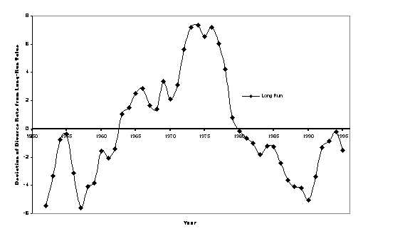
Table 5 reports the coefficients of the normalized cointegrating equation and the corresponding regression statistics for the associated VAR. The estimated coefficients for the female labor force participation rate and the level of median real income are statistically significant at the ten-percent level or better. The cointegrating relation is plotted in Figure 7, which shows that the divorce rate was greater than its long-run level during most of the Sixties and Seventies.
V. Vector error correction and impulse functions
Because the divorce rate, the female labor participation rate, and the level of median real female income are cointegrated, estimation of a vector error correction (VEC) model is the appropriate next step. The vector error correction technique is essentially a restricted VAR that includes the cointegrating equation in the model’s specification. The model is estimated with the data in first difference form, not in levels, and while it allows short-run dynamics, the VEC model includes a restriction that each variable must converge to its long-run, cointegrating relationship.
The parameter estimates of the VEC model are reported in Table 6. While one does not usually emphasize the statistical significance of the individual slope coefficients in a VAR or VEC format, the model’s performance is mixed. The coefficient for the cointegrating equation’s error correction term, which is included in each equation as an explanatory variable, is only statistically significant in the female labor force participation equation. The only significant variable in the divorce equation is the time trend and only the one period lag of the first difference in real income is statistically significant in the income equation. An F-test of the null hypothesis that all slope coefficients are zero is rejected for the divorce and labor force participation equations but not for the income equation.
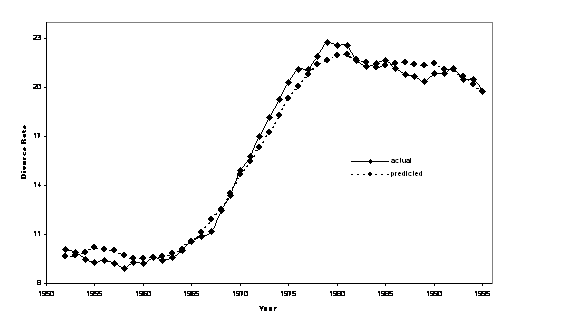
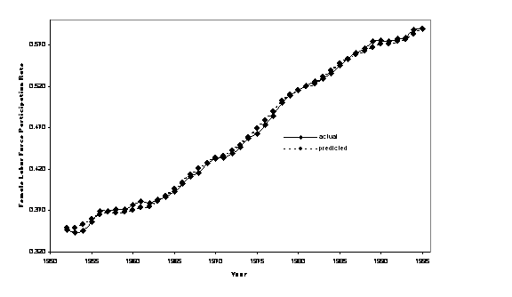
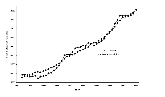
R-squared calculations for these equations vary widely with values ranging from a high of 0.606 for the divorce equation to a low of 0.197 for the income equation. It is important to remember that the dependent variables of these equations are all expressed in first differences. Once the predicted changes in the dependent variables are converted to levels data, the model’s ability to explain variations in the data becomes more apparent. Figure 4 plots the actual and predicted divorce rates in levels data. The R-squared value for this procedure is 0.9902. The actual and predicted levels of the female labor force participation rate are shown in Figure 5, and the close fit is indicative of the level form R-squared of 0.9981. The model also predicts median real female income (in level form) quite well. The actual and predicted values for this variable are plotted in Figure 6, and the recalculated R-squared is 0.9824.
The interpretation of the magnitude, sign and significance of an individual slope coefficient in a VEC model is problematical. After all, the reason for including the lag structure in a VEC model is to eliminate serial correlation, improve forecasting, and avoid misspecification problems when theory is inconclusive about the underlying functional form or the specific set of explanatory variables that should be included. Therefore, it should come as no surprise that a technique other than slope interpretation is used for prediction purposes. [See Stock and Watson, 2001] Consequently, to study the effect of any given change on an explanatory variable, a common practice is to analyze impulse response functions. The impulse response function reveals what happens to a given dependent variable if there is a change or innovation in the error term of one of the other equations in the system. In the results that follow, the innovation in each of the impulse response functions was a one standard deviation increase in the error term of one of the other equations.
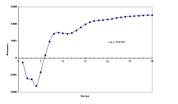
The response of the divorce rate to an increase in the female labor force participation rate is shown in Figure 8. An increase in female labor force participation leads to a decrease in the divorce rate. A very possible explanation for this result is that the wife’s contribution to family income reduces economic pressures on the family and, consequently, decreases the probability of divorce. This is an interesting result when compared to previous studies such as the one by Hannan, Tuma and Groenveld [1978]. It has long been argued that working outside the family contributes to income and income usually contributes to family stability (In the literature, this is referred to as the income effect of female employment). However, a persistent argument has been made that rising female labor force participation increases the female’s level of independence and, along with it, the probability of divorce (In the literature, this is referred to as the independence effect). The evidence produced by this study clearly indicates that an increase in female labor force participation does not increase the likelihood of divorce.
These results are mitigated
somewhat by the impulse response function in Figure 11 which indicates that
increases in female income do lead to rising divorce rates. This finding is in opposition to those
produced by Greenstein [1990] who argues that increases in income contribute to
marital stability. It does appear that
separating the income effect from the independence effect has been problematical. The evidence produced by this study points
to the importance of both the independence effect and the income effect.
Employment may increase martial stability, but higher returns from employment
may result in greater numbers of dissolved marriages.
The impulse response function pictured in Figure 9 reveals that rising divorce rates correspond to rising female labor force participation. There are two probable reasons for this relationship. First, women who have experienced divorce surely enter the labor force in order to offset the loss of income and wealth inevitably associated with marital dissolution. However, another key interpretation of this result is that a rising divorce rate sends a signal to all married females that the probability of remaining married for a lifetime is waning. The appropriate and predictable response is for females to substitute away from nonmarket activities (housework and child rearing) to market activities (work). Greater female investment in human capital is the predictable outcome, and is confirmed by the results provide in Figure 9.
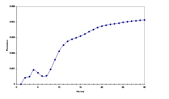
Finally, Figure 10 shows the effect of an
innovation in median female income on labor force participation. Increases in median female income lead to
increases in female labor force participation.
This is not a surprising result.
The incentive to work rises and females respond to the incentive.[8]
VI. Conclusions and
thoughts for future work
Results in this paper indicate that the divorce rate, the female labor force participation rate, and the median level of real female income have unit roots, and that time-series regression with level data may produce spurious results. These variables are integrated of order one, and there exists a single, cointegrating relationship between them. Furthermore, the single cointegrating equation implies that these variables have a single, underlying long-run relationship.
The most interesting results derive from application of impulse response functions to the set of equations. Previous studies on divorce have argued that female labor force participation could have dual effects on marital dissolution. The “income effect” argues that female labor force participation increases income and reinforces familial relationships, thereby leading to a reduction in the likelihood of divorce. A counter argument in the literature focuses on the “independence effect.” This effect hypothesizes that female labor force participation increases income, financial independence and, consequently, the probability of divorce. Time series results from this paper argue for the existence of both effects. Increases in female labor force participation appear to reduce the likelihood of divorce. However, the evidence clearly indicates that increases in female income lead to increases in the likelihood of divorce. Without doubt, income is a much better indicator of financial independence than simple labor force participation.
Bibliography
Becker, Gary S., Elisabeth
M. Landes, and Robert T. Michael, “An Economic Analysis of Martial Instability,
“ Journal of Political Economy, 1977, vol. 85, no.
6, 1141-1187.
Bremmer, Dale and Randy
Kesslering, “The Relationship between Female Labor Force Participation and
Divorce: A Test Using Aggregate Data,” unpublished mimeo, 1999.
Breusch, T.S., “Testing for
Autocorrelation in Dynamic Linear Models,” Australian Economic Papers,
1978, vol. 17, 334-355.
D’amico, Ronald, “Status
Maintenance or Status Competition? Wife’s Relative Wages as a Determinant of
Labor Supply and Martial Instability,” Social Forces, June 1983,
vol. 61, no. 4, 1186-1205.
Dickey, D. A. and W. A.
Fuller, “Distribution of the Estimators for Autoregressive Time Series with a
Unit Root,” Journal of the American Statistical
Association, 1979, vol. 74, 427-431.
Godfrey, L.G., “Testing
against General Autoregressive and Moving Average Error Models When the
Regressors Include Lagged Dependent Variables,” Econometrica, 1978, vol.
46, 1293-1302.
Greene, William H. and Aline
Q. Quester, “Divorce Risk and Wives’ Labor Supply Behavior,” Social Science
Quarterly, March 1982, vol. 63, no. 1, 16-27.
Greenstein, Theodore N.,
“Marital Disruption and the Employment of Married Women,” Journal of
Marriage and the Family, Aug. 1990, vol. 52, no. 3, 657-677.
Hannan, Michael T., Nancy
Brandon Tuma and Lyle P. Groenveld, Income and
Hoffman, Saul and Greg Duncan,
“The Effect of Incomes, Wages, and AFDC Benefits on Martial Disruption,” The
Journal of Human Resources, vol. 30, no. 1, 19-41.
Johansen, Soren, and
Katarina Juselius, “Maximum Likelihood Estimation and Inferences on
Cointegration – with Applications to the Demand for Money,”
Johansen, Soren, “Estimation
and Hypothesis Testing of Cointegrated Vectors in Gaussian Vector
Autoregressive Models,” Econometrica, vol. 59, 1551-1580.
Johnson, William R. and
Jonathan Skinner, “Labor Supply and Martial Separation,” American Economic
Review, June 1986, vol. 76, no. 1, 455-469.
Lombardo, Karen V., “Women’s
Rising Market Opportunities and Increased Labor Force Participation,” Economic
Inquiry, April 1999, vol. 37, no. 2, 195-212.
Mincer, Jacob, “Intercountry
Comparisons of Labor Force Trends and Related Developments: An Overview,” Journal
of Labor Economics, 1985, vol. 3, no. 1, pt. 2, S1-32.
Nelson, C. R. and C. I.
Plosser, “Trends and Random Walks in Macroeconomic Time Series: Some Evidence
and Implications,” Journal of Monetary Economics, 1982,
vol. 10, 139-162.
Shapiro, David and Lois
Shaw, “Growth in Supply Force Attachment of Married Women: Accounting for
Changes in the 1970's,” Southern Economic Journal,
September 1985, vol. 6, no. 3, 307-329.
South, Scott,
“Economic Conditions and the Divorce Rate: A Time-Series Analysis of Postwar
United States,” Journal of Marriage and the Family,
February 1985, vol. 47, no. 1, 31-41.
South, Scott
and Glenna Spitze, “Determinants of Divorce over the Martial Life Course,” American
Sociological Review, August 1986, vol. 51, 583-590.
Spitze,
Glenna, and Scott South, “Women’s Employment, Time Expenditure, and Divorce,” Journal
of Family Issues, September 1985, vol. 6, no. 3, 307-329.
Stock, James
H. and Mark W. Watson, “Vector Autoregressions,” Journal of Economic
Perspectives, Fall 2001, vol. 15, no. 4, 101-115.
