The Impact of Defense Spending on GDP:
The Case of
by
Dale
Bremmer
Professor of Economics
Department of Humanities and Social Sciences
Rose-Hulman Institute of Technology
and
Randy
Kesselring
Professor of Economics
Department of Economics and Finance
April
2007
Presented During the “Topics in Economics” Session
at the 49th Annual Conference of the
Western Social Science Association
Hyatt Regency Hotel,
Friday, April 13,
2007, 8:00 a.m. – 9:30 a.m.
The Impact of Defense Spending on Economic
Growth: The Case of
I. Introduction
With
the demise of the Soviet Union in the early 1990s, the fall of the Berlin Wall
and the end of the Cold War, some saw the need for decreased military spending
by the
This
paper is a pilot study which examines whether increases in military spending have
a positive or negative impact on a country’s GDP. The study focuses on the three North American
economies:
The
results produced by the statistical models are asymmetric. Increased military spending in
The rest of the paper is organized as follows. Following this introduction, the second section of the paper provides a brief review of the past literature regarding the impact of defense spending on a country’s economy. A description of the empirical model and the data is found in the third section of the paper. This section also contains a discussion of the unit root tests and an analysis of the pairwise Ganger-causality tests. The empirical results and the impulse response functions are analyzed in the fourth section, while the final section of the paper offers a critique of the results and some ideas for future research.
II.
Literature
Review
Previous papers on
the impact of a nation’s defense spending on its economy have concentrated on four
areas. Some researchers have stressed
the relationship between military spending and private investment. Others (especially development economists)
have investigated the effect that defense spending has on employment. Still others have investigated an economy’s demand
for defense expenditures. Finally, the
most common approach has been to relate military spending directly to the
nation’s ability to produce output (GDP).[1] The literature review that follows has been
divided into these four areas.
The impact of defense spending on private investment
Several studies have concluded that, in the case of developed nations, investment and military expenditures are substitutes (Kennedy 1983, p. 198). Smith (1977, 1978, 1980, and 1983) argues that households are very resistant to cuts in private consumption and public welfare. Given an exchange rate and a level of capacity utilization, the remainder of the nation’s output is divided between defense spending and investment. The result is that a higher level of military spending leads to a lower level of investment. In a study of 15 countries between 1960 and 1970, Smith found that investment spending and defense spending were negatively correlated (-0.73). Lindgren (1984) points out that most studies are in agreement on the negative correlation between defense spending and investment spending for industrialized, market economies.
More recently, a
study by Laopodis (2001) produced substantially different results. Using Granger causality tests on a
time-series of data (1960-1997) for
The impact of defense spending on employment
Regarding the impact of military expenditures on employment, the Marxist critique of the 1960s was that defense spending was a necessary, albeit wasteful, policy to stabilize and expand capitalism (Baran and Sweezy 1968). They argued that by raising the level of defense spending a country could solve the problems of under consumption and the unemployment associated with it. Furthermore, capitalism would resort to such spending in an effort to reduce class conflict. The hypothesis that increased military spending indirectly creates employment in the armaments industry and directly creates more jobs in the armed forces does not necessarily need to rely on the tenants of Marxist economics for support. Indeed, one of the primary concerns regarding disarmament at the end of the Cold War was its hypothesized relationship to rising unemployment.
In spite of this
intuitive relationship,
An interesting approach to this estimation problem was provided by Hooker and Knetter (1997). Using a panel data model for the U.S, they found that defense procurement spending which does vary from state to state had a significant impact on statewide employment. Both the time series and the cross sections were accounted for with fixed effects. Additional evidence was produced that the effects of defense spending on employment are decidedly nonlinear with larger changes in defense spending produce significantly greater changes in employment.
Several other
research efforts have been focused on specific countries. Wing (1991), using input-output analysis,
found that defense spending had a significant impact on employment in
The Demand for Defense Expenditures
Another interesting facet of research on military expenditures is the question of demand determination. Early researchers in this area tended to estimate demand specifications for defense spending that were closely related to standard household demand theory. Hartley and Sandler (1990) provide a good review of these studies. The results seem to indicate that defense spending is a normal good (positively related to GDP) and that, being a public good, there is significant free riding.
Sandler and Murdoch (1991) add elements of game theory to the formulation of demand models for defense expenditure. Murdoch et al (1991) test what is referred to as a median voter demand model against an oligarchy model for members of NATO and get mixed results. Hanson et al. (1990), Hilton and Vu (1991) and Conybeare et al. (1994) all test empirical models of defense demand concentrating on NATO countries. While all of these authors use slightly different approaches they tend to get similar results regarding income or GDP (defense provision is a normal good) and produce mixed results about free riding. They also tend to agree that degree of external threat is an important determinant of demand.
A recent paper by Solomon (2005)
uses a kind of cointegration technique (autoregressive distributed lag
approach) to investigate the demand for military spending in
The Impact of Defense Spending On GDP
Given the long-accepted, theoretical direct relationship between investment and economic growth, if defense spending has a negative impact on investment, then it would seem reasonable that defense spending would have an adverse impact on economic growth. This was exactly the findings of two studies published in the seventies, Szymanski (1973) and Lee (1973). Some studies attribute the negative effect of defense spending on economic growth to reduced investment.[2] Another study argues that defense spending restricts export growth and economic growth because military expenditures compete for the same resources used in the production of exports.[3]
However, other
studies were unable to find any stable relationship between military spending
and economic growth.[4]
Perhaps because of
the above criticisms, models based on seemingly sounder theoretical development
have come into common use by researchers of this relationship. One of these models is generally referred to
as the Feder-Ram model because it was adapted by Biswas and Ram (1986) from an
export model developed by Feder (1983). Cuaresma
and Reitschuler (2003) used a version of this model for the
A number of recent
papers have attacked the problem through application of a type of Granger
causality estimation. Because they use
Granger causality these papers generally limit their analysis to examination of
only two variables, defense spending and GDP. Dakurah et al. (2001) examined 62 less developed countries (LDCs) with data
from 1975 to 1995. A type of two-way
Granger causality was estimated for all of the countries. Only 23 countries exhibited unidirectional
causality, and in 16 of those 23 the relationship between defense spending and
GDP was positive. For the remaining 7,
the relationship was negative. But, for
most of the countries, there was no relationship. Karagol and Palaz (2004) applied a similar
technique to
Atesoglu (2002)
formulates a multivariable reduced-form Keynesian model patterned after Romer
(2000). Using cointegration estimation
techniques for the years 1947 to 2000, Atesoglu finds a positive long-run
relationship between military spending and output for the
Obviously, the
results from many different models estimated in several different ways have
been mixed. Consequently, the search is
still on for a model and an estimation technique that will provide consistent
results. Our attempt begins by looking
at the entire process in a slightly different way. Economists are always concerned about policy
making and, therefore, policy variables.
Governments have at their disposal several tools with which to affect
the macro economy. These tools are
usually divided into two classes: monetary and fiscal policy tools. Obviously, control over military spending is
a “fiscal” policy tool. So, our approach
is to use military spending within a model that was originally set forth to
distinguish the effectiveness of these tools—the
III. The Model, the Data,
Unit Root Tests, and Granger-Causality Tests
To determine the
relative impacts of defense spending, other central government spending and
monetary policy on a country’s output, a “![]() equal the annual percentage change in nominal GDP that was
observed in year t. To distinguish
between the change in defense spending and other central government
expenditures, let
equal the annual percentage change in nominal GDP that was
observed in year t. To distinguish
between the change in defense spending and other central government
expenditures, let ![]() denotes the annual
percentage change in nominal military expenditures in year t, while
denotes the annual
percentage change in nominal military expenditures in year t, while ![]() equals the percentage change in nominal nonmilitary
expenditures in year t. Finally, to
control for the differences between fiscal and monetary policy,
equals the percentage change in nominal nonmilitary
expenditures in year t. Finally, to
control for the differences between fiscal and monetary policy, ![]() is the annual percentage change in the nominal money supply
in year t.
is the annual percentage change in the nominal money supply
in year t.
Specifying the VAR model
The vector autoregression (VAR) model is a seemingly unrelated system of four regressions where each of the current dependent variables is a function of lagged dependent variables. The VAR model below assumes that each regression has the same lag structure or
![]() (1)
(1)
![]() (2)
(2)
![]() (3)
(3)
and
![]() (4)
(4)
On the right-hand side of each equation, T lags of each dependent variable are used as explanatory variables. Also notice that the right-had sides of Equations (1)-(4) contain no other exogenous explanatory variables.
The data
To
initially test the impact of military spending on the growth rate of GDP, this
paper used a pilot case of the three North American countries:
Table
1 shows that the military expenditures in the
Between
1963 and 2005, military expenditures as a percentage of GDP fell for each of
the three countries. As Table 1 shows, almost
during the height of the Vietnam War, military spending was 9.09 percent of GDP
in the
The unit root tests
Regressions
with time series data run the risk of obtaining spurious results. This occurs when regressions estimated with
one or more nonstationary data series result in statistically significant results
even though there may be no true underlying relationship. To avoid spurious results, augmented
Dickey-Fuller tests are performed on each data series to determine whether the
data exhibit unit roots and are nonstationary.
The results of the augmented Dickey-Fuller tests are reported in Table
2. The four data series are annual
percentage changes in GDP, military spending, other expenditures of the central
government, and the money supply. Table
2 lists the results of the unit root tests on these series for
In
the case of
According to the results in Table 2, the percentage change in Mexican GDP and the percentage change in Mexican military spending are nonstationary in levels, but stationary in first differences. However, in the case of the percentage change in other spending by the Mexican central government, the null hypothesis of a zero root is rejected at the one percent level while the null hypothesis that the percentage change in the Mexican money supply has a zero root can be rejected at the five percent level. The unit root tests indicate that the first differences of the percentage changes in Mexican money supply and other central government expenditures are stationary. Because statistical data indicate that level data of at least two of the four series data exhibit nonstationarity, the Mexican data will have to be estimated in first differences and cointegration test have to be performed.
Finally,
level forms of the
Pairwise Granger-causality tests
Pairwise Granger-causality test are reported in Table 3. These statistical tests investigate whether changes in GDP causes changes in military spending or does changes in military spending causes changes in GDP. For each of the three countries, these tests involved estimating two simple linear regressions, one having the percentage change in GDP as the dependent variable and the other having the percentage change in military spending as the dependent variable. The explanatory variables of these regressions are lagged values of the percentage changes in military spending and GDP. The number of lags was determined by picking that model specification that minimized the Akaike Information Criterion (AIC).
In
the case of
However, the
opposite result was found for the
IV. Estimation Results of
the VAR Model and Impulse Response Functions
The
VAR models are estimated for
Estimation of the Canadian, Mexican and
Tests indicate that only one lag was needed in the Canadian VAR model. The main advantage of using the VAR framework is its a-theoretic, reduced-form framework that doesn’t require careful specification of a structural model and its comparative advantage in forecasting. Given the reduced-form structure of the model, interpreting the signs and the statistical significance and the sign of an individual coefficient becomes more problematic. Since the Canadian data was stationary, the results in Table 4 were obtained using levels data. The results in Table 4 indicate that only one of the four regression models have a significant F-statistic. Estimation results indicate that null hypothesis that all the slope coefficients are simultaneously zero is rejected at the five percent level for the regression model with the GDP growth rate as a dependent variable.
Since the unit root tests indicated that Mexican data was nonstationary, cointegration tests were performed and their results are reported in Table 5. Using the techniques developed by Johansen, both the trace test and the maximum-eigenvalue test indicate the presence of at most one cointegrating equation with an intercept present.[6] Having determined the presence of one cointegrating equation and its underlying structure, an error-corrected VAR model was estimated and the results are listed in Table 6. All four of the regressions reported in Table 6 have significant F-tests implying that none of the models have slope coefficients that are simultaneously zero.
The
estimation results for the
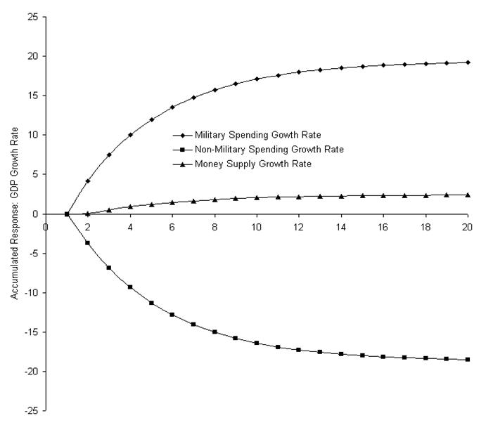
The impulse response functions
The
impulse functions of the three VAR models are shown in Figures 1, 2, and
3. The Canadian results are shown in
Figure 1, the Mexican results are depicted in Figure 2 and Figure 3 shows the
The response of the growth rate of Canadian GDP to a shock in the other variables is shown in Figure 1. The estimation results indicate that positive innovations to either the growth rate in military spending and money supply lead to increases in the growth rate of GDP. However, if the Canadian federal government increases the growth rate of other spending Canadian GDP falls.
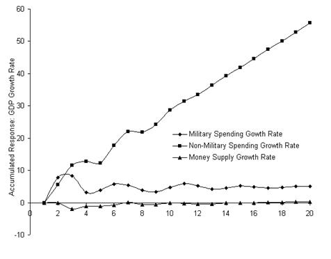
According to the information in Figure 2, positive innovations to government expenditures, either military or nonmilitary, lead to increases in Mexican GDP. But, Mexican monetary policy almost appears neutral as a positive innovation in the nominal money supply has little long-run effect on the growth rate of Mexican GDP.
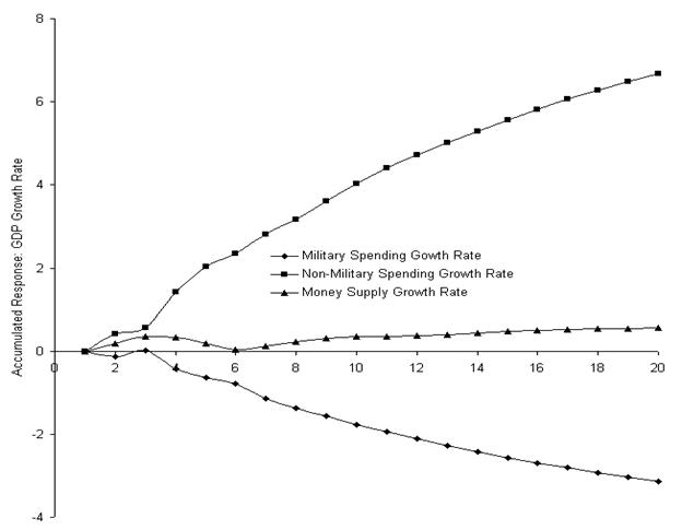
While
Canadian and Mexican military spending stimulate GDP growth in their respective
countries, Figure 3 shows that an increase in the growth rate of military
expenditures in the
V. Conclusion
Both pairwise
Granger-causality tests and impulse response functions from VAR models show an
asymmetric response of the growth rate in GDP of the North American countries
to a change in military spending.
Increased military spending increases nominal GDP in
The
results of the paper foreshadow a threshold effect in that military spending in
the
The
use of a “
Future work will extend this analysis to more countries. The countries will differ in economic development and the size of military spending. Depending on data availability, a tax variable should be added to control for another tool of fiscal policy. Data sets with quarterly data will also be analyzed, but quarterly data on defense spending by developing countries is difficult to obtain.
Economics
is the “Dismal Science” and the forecast of the model in this paper is
bleak. Military spending in the
References
Ahmed, S. “Temporary and Permanent Government Spending in an Open Economy,” Journal of Monetary Economics, 17, 2, 1986, pp. 405-419.
Atesoglu,
H. Sonmez, “Defense Spending Promotes Aggregate Output in the
Baran, Paul and Paul Sweezy. Monopoly Capital. Harmondsworth: Penquin, 1968.
Biswas, B and R. Ram, “Military Expenditure and Economic Growth in Less Developed Countries: An Augmented Model and Further Evidence,” Economic Development and Cultural Change, 34, 1986, pp. 361-372.
Blackaby, Frank and Thomas Ohlson. “Military Expenditure and Arms Trade: Problems of Data,” Bulletin of Peace Proposals, 13, 4, 1982, pp. 291-308.
Bremmer,
Dale and
Cappelen, Adne, Nils Petter Gleditsch and Olav Bjerkholt. “Military Spending and Economic Growth in the OECD Countries,” Journal of Peace Research, 21, 4, 1984, pp. 375 - 387.
Chowdhury, Abdur. “A Causal Analysis of Defense Spending and Economic Growth,” Journal of Conflict Resolution, 35, 1, 1991, pp. 80-97.
Conybeare, J.A.C., J.C. Murdoch and T. Sandler, “Alternative Collective-Goods Models of Military Alliances—Theory and Empirics,” Economic Inquiry, 32, 4, 1994, pp. 525-542.
Cuaresma,
Jesus Crespo and Gerhard Reitschuler, “A Non-Linear Defence-Growth Nexus?
Evidence from the
Dakurah, A. Henry, Stephen P. Davies and Rahan K. Sampath, “Defense Spending and Economic Growth in Developing Countries: A Causality Analysis,” Journal of Policy Modeling, 23, 2001, pp. 651-658.
De
Grasse Jr., Robert W. Military Expansion Economic Decline:
The Impact of Military Spending on
Deger, S., “Economic Development and Defence Expenditure,” Economic Development and Cultural Change, 35, 1, 1986, pp. 179-196.
Dunne, P. and R. Smith. “Military Expenditure and Unemployment in the OECD,” Defense Spending, 1, 1990, pp. 57-73.
Dunne, Paul J., Ron P. Smith and Dirk Willenbockel, “Models of Military Expenditure and Growth: A Critical Review,” Defence and Peace Economics, 16, 6, 2005, pp. 449-461.
Faini, Riccardo, Patricia Annez, and Lance Taylor. “Defense Spending , Economic Structure and Growth: Evidence Among Countries and Over Time,” Economic Development and Cultural Change, 32, 3, 1984, pp. 487-498.
Feder, G., “On Exports and Economic Growth,” Journal of Development Economics, 12, 1983, pp. 59-73.
Galvin, Hannah, “The Impact of Defence Spending on the Economic Growth of Developing Countries: A Cross-Section Study,” Defence and Peace Economics, 14, 1, 2003, pp. 51-59.
Hanson, L., J.C. Murdoch and T. Sandler, “On Distinguishing the Behavior of Nuclear and Non-nuclear Allies in NATO,” Defence Economics, 1, 1, 1990, pp. 37-55.
Hartley,
K. and T. Sandler (eds.), The Economics
of Defence Spending: An International Survey,
Hausman, J. "Specification Tests in Econometrics," Econometrica, 46, 1978, pp. 1251-1271.
Hilton,
B., and A. Vu, “The McGuire Model and the Economics of the NATO
Hooker, Mark A. and Michael M. Knetter, “The Effects of Military Spending on Economic Activity: Evidence from State Procurement Spending,” Journal of Money, Credit, and Banking, 29, 3, 1997, pp. 400-421.
Huang,
Jr-Tsung, and An-Pang Kao, “Does Defence Spending Matter to Employment in
Judge,
George G., R. Carter Hill, William E. Griffiths, Helmut Lütkepohl, and
Tsoung-Chao Lee. Introduction to
the Theory and Practice of Econometrics.
Karagol,
Erdal and Serap Palaz, “Does Defence Expenditure Deter Economic Growth in
Kennedy,
Gavin. Defense Economics.
Klein, Thilo,
“Military Expenditure and Economic Growth:
Kollias,
Christos, Charis Naxakis and Leonidas Zarangas, “Defence Spending and Growth in
Laopodis, Nikiforos T., “Effects of Government Spending on Private Investment,” Applied Economics, 33, 2001, pp. 1563-1577.
Lee,
Jong Ryol. “Changing National Priorities of the
Lindgren, Göran. “Armaments and Economic Performance in Industrialized Market Economies,” Journal of Peace Research, 21, 4, 1984, pp. 375-387.
Murdoch,
J.C., T. Sandler and L. Hansen, “An Econometric Technique for Comparing Median
Voter and Oligarchy Choice Models of Collective Action—the Case of the NATO
Nardinelli, Clark and Gary B. Ackerman. “Defense Expenditures and the Survival of American Capitalism,” Armed Forces and Society, 3, 1, 1976, pp. 13-16.
Paul, Satya. “Defense Spending and Unemployment Rates: An Empirical Analysis for the OECD,” Journal of Economic Studies, 23, 2, 1996, pp. 44-54.
Romer, David, “Keynesian Macroeconomics Without the LM Curve,” Journal of Economic Perspectives, 14, 2, 2000, pp. 149-169.
Rotschild, Kurt W. “Military Expenditure, Exports, and Growth,” Kyklos, 26, 4, 1973, pp. 804-813.
Sandler, T., and J.C. Murdoch, “Nash-Cournot or Lindahl Behavior? An Empirical Test for the NATO Allies,” Quarterly Journal of Economics, 105, 4, 1991, pp. 875-894.
Smith,
Ron P. “Military Expenditure and Capitalism,”
Smith,
Ron P. “Military Expenditure and Capitalism: A Reply,”
Smith, Ron P. “Military Expenditure and Investment in OECD Countries, 1954-1973,” Journal of Comparative Economics, 4, 1980, pp. 19-32.
Smith Ron P. and George Georgiou. “Assessing the Effect of Military Expenditure on OECD Economies: A Survey,” Arms Control, 14, 1, 1983, pp. 3-15.
Solomon, Binyam, “The Demand for Canadian Defence Expenditures,” Defence and Peace Economics, 16, 3, 2005, pp. 171-189.
Szymanski, Albert. “Military Spending and Economic Stagflation,” American Journal of Sociology, 79, 1, 1973, pp. 1-14.
Weede, Erich 1983. “Military Participation rations, Human Capital Formation, and Economic Growth: A Cross-national Analysis,” Journal of Political and Military Sociology, 11(Spring), 11-19.
Wing,
M.M., “Defense Spending and Employment in
Yildirim,
J. and S. Sezgin, “A System Estimation of the Defence-Growth Relation in
Yildirim, J., Selami Sezgin and Nadir Ocal, “Military Expenditure and Economic Growth in Middle Eastern Countries: A Dynamic Panel Data Analysis,” Defence and Peace Economics, 16, 4, 2005, pp. 283-295.
Table 1: Military Expenditures as a Percent of Central Government Expenditures and GDP:
|
Military Expenditures as a Percent of Central Government Expenditures |
|
Military Expenditures as a Percent of GDP |
||||||
|
Year |
|
|
|
|
Year |
|
|
|
|
1963 |
24.03 |
9.86 |
49.15 |
|
1963 |
3.56 |
0.72 |
8.47 |
|
1964 |
22.90 |
9.64 |
46.22 |
|
1964 |
3.44 |
0.72 |
7.72 |
|
1965 |
22.60 |
10.00 |
44.05 |
|
1965 |
3.16 |
0.71 |
7.20 |
|
1966 |
22.11 |
9.93 |
46.87 |
|
1966 |
3.11 |
0.72 |
8.07 |
|
1967 |
18.70 |
8.10 |
49.40 |
|
1967 |
3.11 |
0.68 |
9.09 |
|
1968 |
16.30 |
8.10 |
45.20 |
|
1968 |
3.10 |
0.69 |
8.87 |
|
1969 |
11.60 |
6.60 |
44.10 |
|
1969 |
2.62 |
0.70 |
8.27 |
|
1970 |
12.90 |
6.80 |
39.80 |
|
1970 |
2.39 |
0.70 |
7.50 |
|
1971 |
11.60 |
7.60 |
35.20 |
|
1971 |
2.23 |
0.73 |
6.64 |
|
1972 |
10.50 |
4.90 |
33.40 |
|
1972 |
2.03 |
0.99 |
6.27 |
|
1973 |
9.70 |
4.40 |
30.10 |
|
1973 |
1.83 |
0.88 |
5.67 |
|
1974 |
8.50 |
4.30 |
30.30 |
|
1974 |
1.68 |
0.43 |
5.73 |
|
1975 |
7.70 |
4.40 |
26.20 |
|
1975 |
1.57 |
0.56 |
5.55 |
|
1976 |
8.20 |
3.90 |
23.60 |
|
1976 |
1.34 |
0.54 |
4.99 |
|
1977 |
8.70 |
3.90 |
23.80 |
|
1977 |
1.62 |
0.44 |
4.97 |
|
1978 |
8.70 |
2.80 |
23.00 |
|
1978 |
1.92 |
0.36 |
4.76 |
|
1979 |
8.20 |
2.70 |
23.30 |
|
1979 |
1.83 |
0.33 |
4.77 |
|
1980 |
8.50 |
2.10 |
23.10 |
|
1980 |
1.92 |
0.23 |
5.16 |
|
1981 |
7.80 |
2.30 |
23.60 |
|
1981 |
1.84 |
0.32 |
5.43 |
|
1982 |
8.10 |
1.50 |
25.00 |
|
1982 |
2.14 |
0.48 |
6.03 |
|
1983 |
7.90 |
2.00 |
25.50 |
|
1983 |
1.78 |
0.69 |
6.16 |
|
1984 |
8.20 |
2.70 |
26.40 |
|
1984 |
1.87 |
0.79 |
7.14 |
|
1985 |
8.60 |
2.60 |
25.70 |
|
1985 |
2.02 |
0.58 |
6.12 |
|
1986 |
9.20 |
2.30 |
27.10 |
|
1986 |
2.07 |
0.86 |
6.29 |
|
1987 |
9.30 |
2.30 |
27.20 |
|
1987 |
1.93 |
1.18 |
6.08 |
|
1988 |
9.30 |
2.10 |
26.20 |
|
1988 |
1.70 |
0.69 |
5.74 |
|
1989 |
7.10 |
2.50 |
25.50 |
|
1989 |
1.31 |
0.65 |
5.54 |
|
1990 |
7.00 |
2.60 |
23.50 |
|
1990 |
1.33 |
0.54 |
5.27 |
|
1991 |
6.30 |
4.30 |
19.60 |
|
1991 |
1.26 |
0.52 |
4.67 |
|
1992 |
6.20 |
4.60 |
21.10 |
|
1992 |
1.33 |
0.51 |
4.81 |
|
1993 |
6.90 |
4.00 |
19.90 |
|
1993 |
1.53 |
0.52 |
4.48 |
|
1994 |
6.70 |
4.70 |
18.80 |
|
1994 |
1.51 |
0.63 |
4.07 |
|
1995 |
6.40 |
3.90 |
17.40 |
|
1995 |
1.38 |
0.81 |
3.77 |
|
1996 |
6.00 |
3.60 |
16.50 |
|
1996 |
1.23 |
0.67 |
3.47 |
|
1997 |
5.80 |
3.60 |
16.30 |
|
1997 |
1.12 |
0.62 |
3.32 |
|
1998 |
5.90 |
3.80 |
15.80 |
|
1998 |
1.28 |
0.60 |
3.13 |
|
1999 |
5.90 |
3.74 |
15.70 |
|
1999 |
1.26 |
0.56 |
3.03 |
|
2000 |
5.77 |
3.34 |
16.18 |
|
2000 |
1.15 |
0.52 |
3.07 |
|
2001 |
6.10 |
3.49 |
15.88 |
|
2001 |
1.17 |
0.54 |
3.09 |
|
2002 |
6.09 |
3.09 |
16.98 |
|
2002 |
1.15 |
0.50 |
3.41 |
|
2003 |
6.04 |
2.84 |
18.44 |
|
2003 |
1.15 |
0.46 |
3.79 |
|
2004 |
5.93 |
2.55 |
19.50 |
|
2004 |
1.14 |
0.41 |
3.97 |
|
2005 |
5.86 |
2.41 |
19.84 |
|
2005 |
1.12 |
0.39 |
4.07 |